
Trade-offs in Explanatory Model Learning DCAP



Description: Trade-offs in Explanatory Model Learning DCAP Meeting Madalina Fiterau 22nd of February 2012 1 Outline Motivation: need for interpretable models Overview of data analysis tools Model evaluation accuracy vs complexity Model evaluation
Related Topics
Download Presentation
"Trade-offs in Explanatory Model Learning DCAP" is the property of its rightful owner. Permission is granted to download and print the materials on this website for personal, non-commercial use only, and to display it on your personal computer provided you do not modify the materials and that you retain all copyright notices contained in the materials. By downloading content from our website, you accept the terms of this agreement.
Presentation Transcript
slide1. Trade-offs in Explanatory
Model Learning DCAP Meeting
Madalina Fiterau 22nd of February 2012 1<br>
slide2. Outline Motivation: need for interpretable models
Overview of data analysis tools
Model evaluation – accuracy vs complexity
Model evaluation – understandability
Example applications
Summary 2<br>
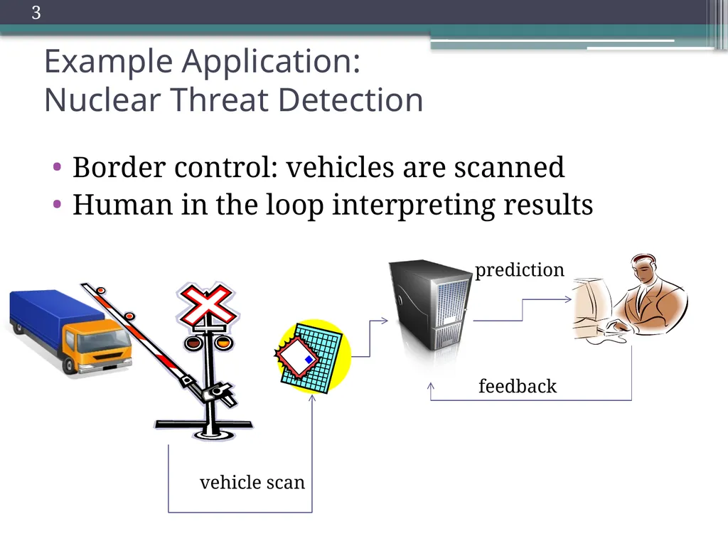
slide3. Example Application: Nuclear Threat Detection Border control: vehicles are scanned
Human in the loop interpreting results vehicle scan prediction feedback 3<br>
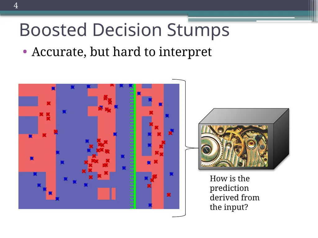
slide4. Boosted Decision Stumps Accurate, but hard to interpret How is the prediction derived from the input? 4<br>
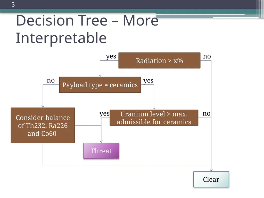
slide5. Decision Tree – More Interpretable Radiation > x% Payload type = ceramics Uranium level > max. admissible for ceramics Consider balance of Th232, Ra226 and Co60 Clear yes no yes no Threat yes no 5<br>
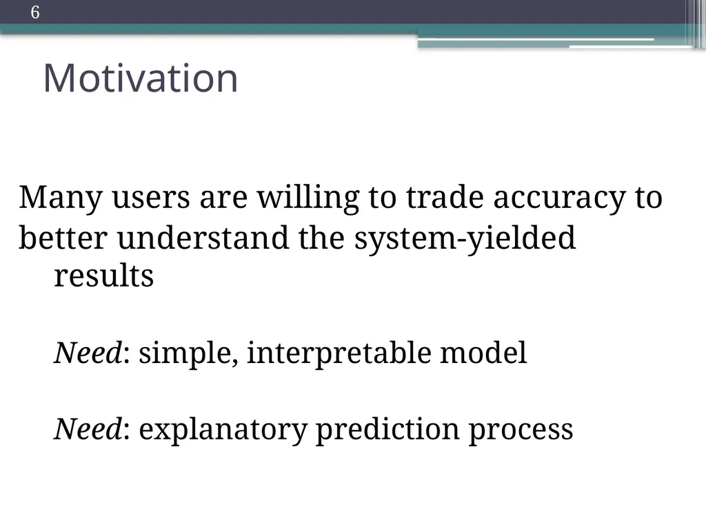
slide6. Motivation 6 Many users are willing to trade accuracy to
better understand the system-yielded results
Need: simple, interpretable model
Need: explanatory prediction process<br>
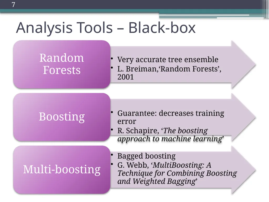
slide7. Analysis Tools – Black-box 7<br>
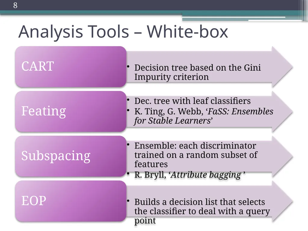
slide8. Analysis Tools – White-box 8<br>
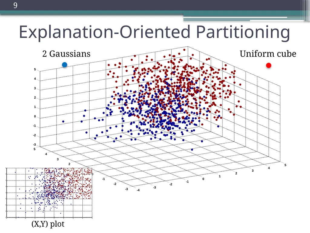
slide9. Explanation-Oriented Partitioning (X,Y) plot 9<br>
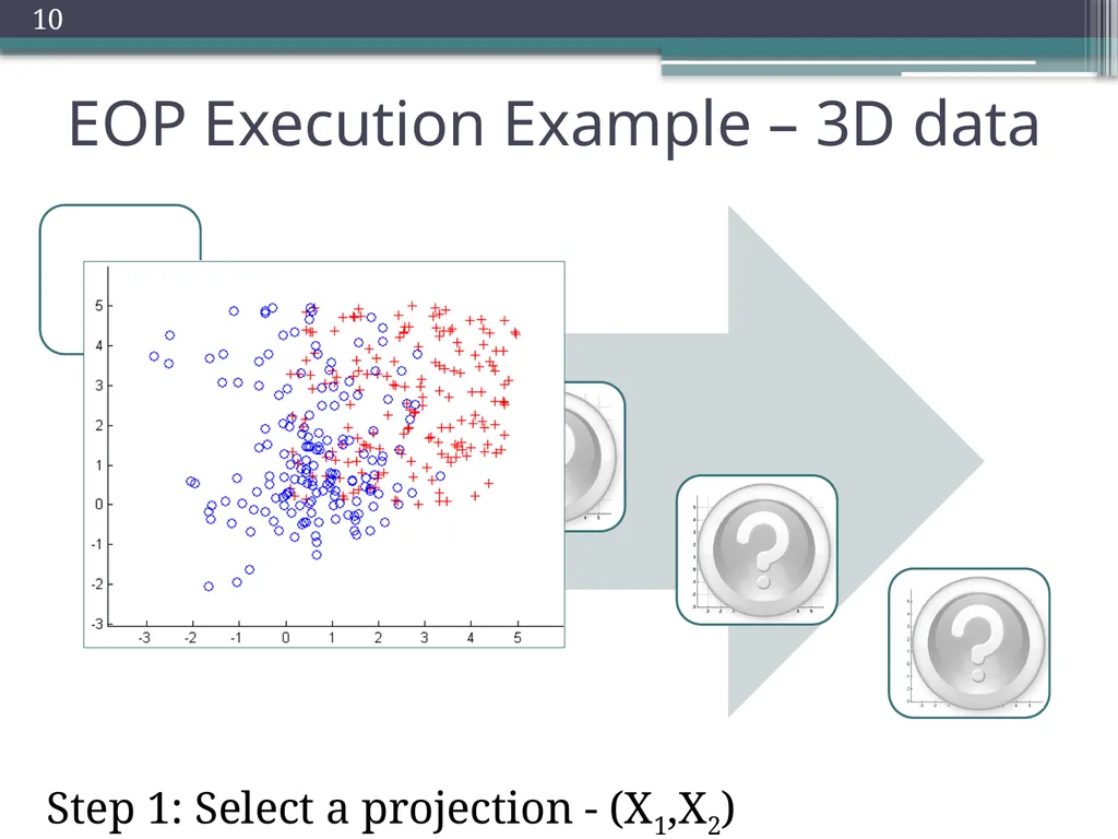
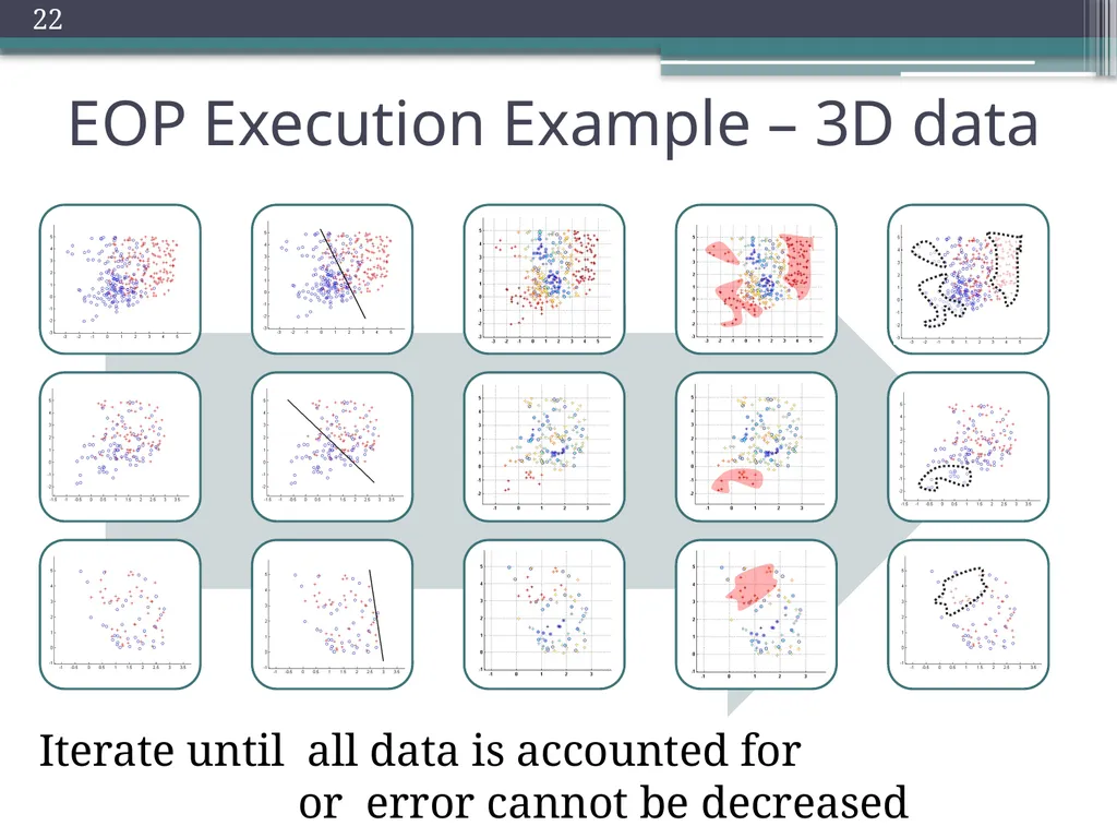
slide10. EOP Execution Example – 3D data Step 1: Select a projection - (X1,X2) 10<br>
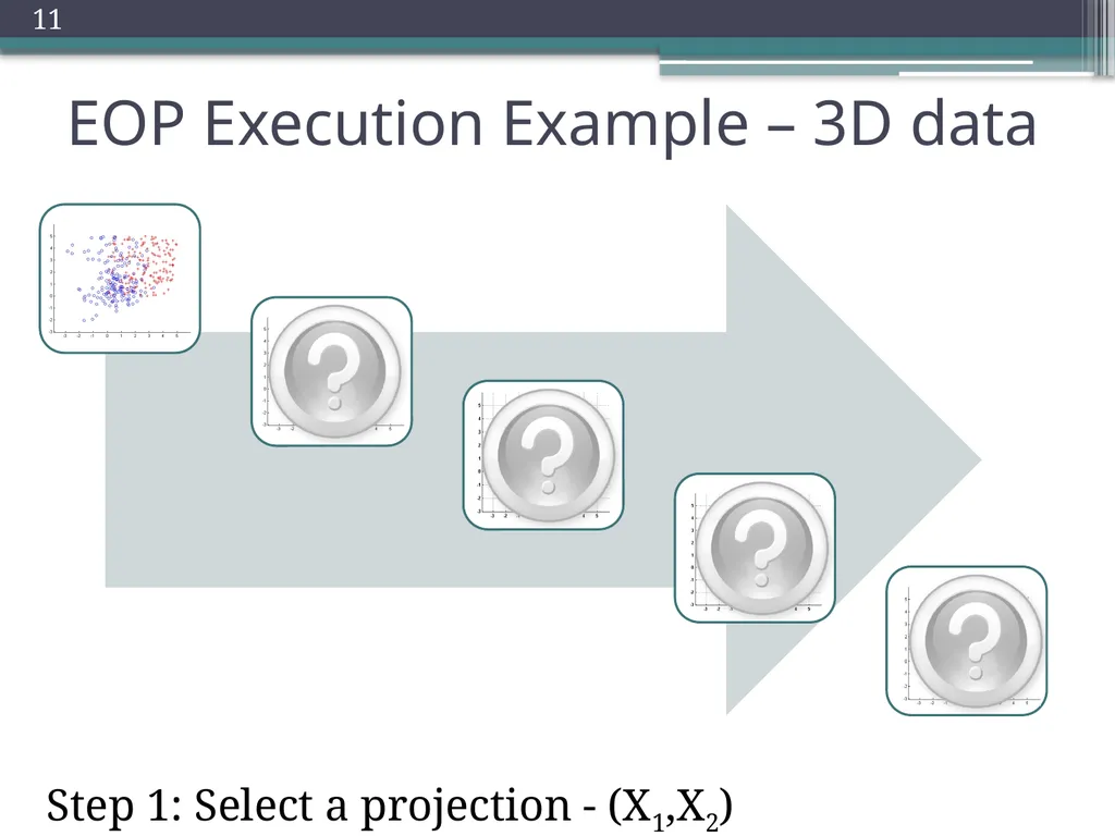
slide11. Step 1: Select a projection - (X1,X2) 11 EOP Execution Example – 3D data<br>
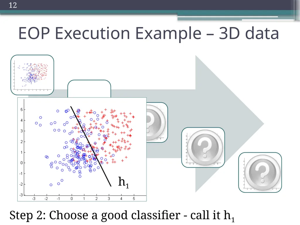
slide12. Step 2: Choose a good classifier - call it h1 h1 12 EOP Execution Example – 3D data<br>
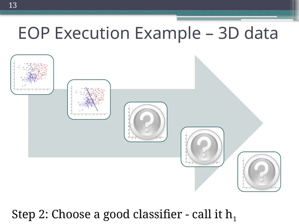
slide13. Step 2: Choose a good classifier - call it h1 13 EOP Execution Example – 3D data<br>
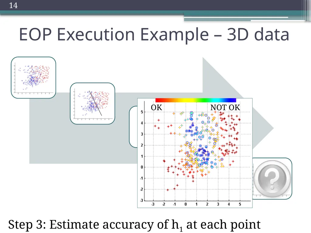
slide14. Step 3: Estimate accuracy of h1 at each point 14 EOP Execution Example – 3D data<br>
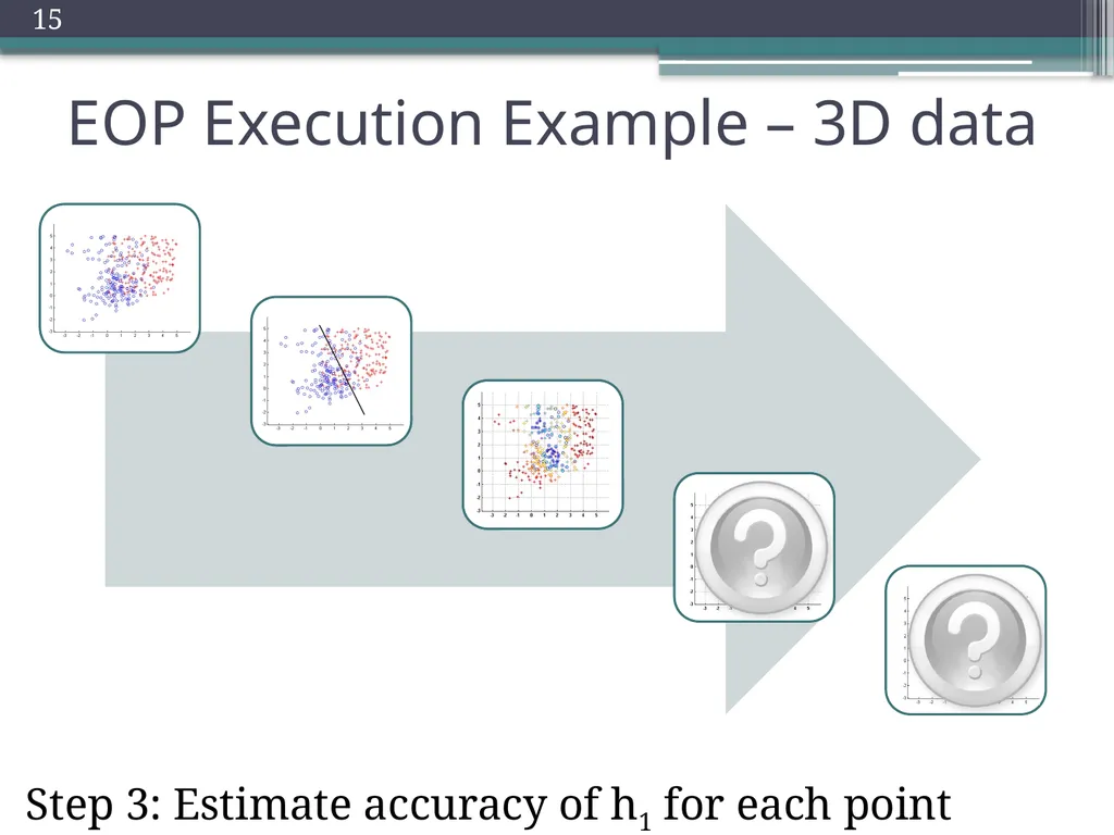
slide15. Step 3: Estimate accuracy of h1 for each point 15 EOP Execution Example – 3D data<br>
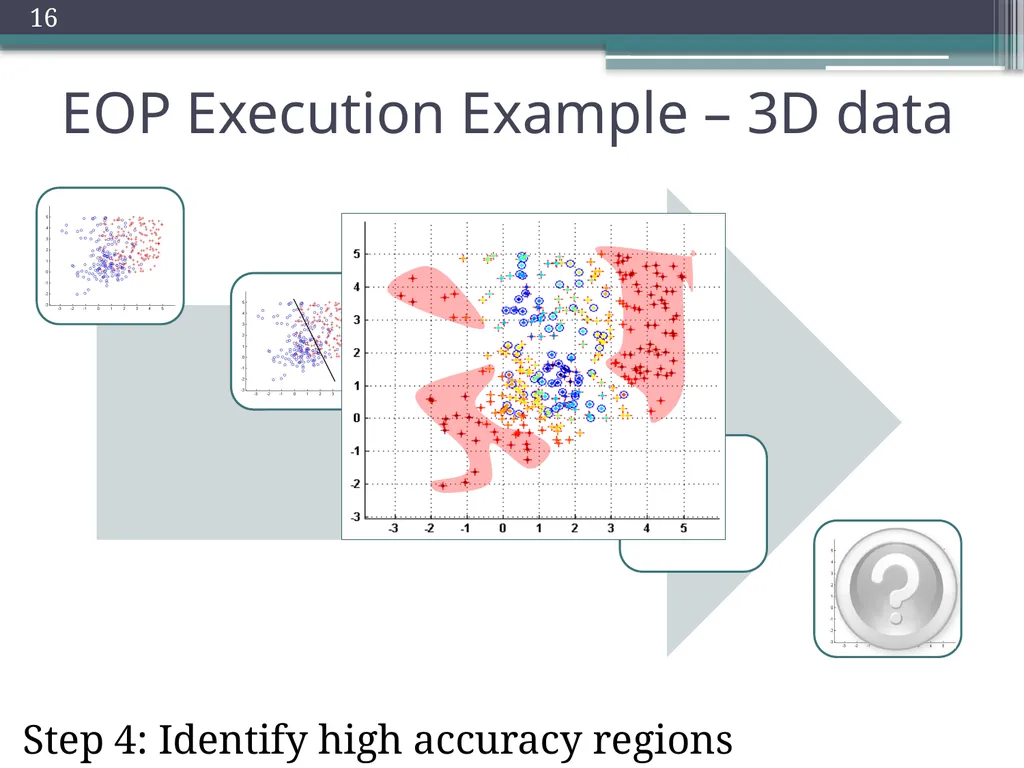
slide16. Step 4: Identify high accuracy regions 16 EOP Execution Example – 3D data<br>
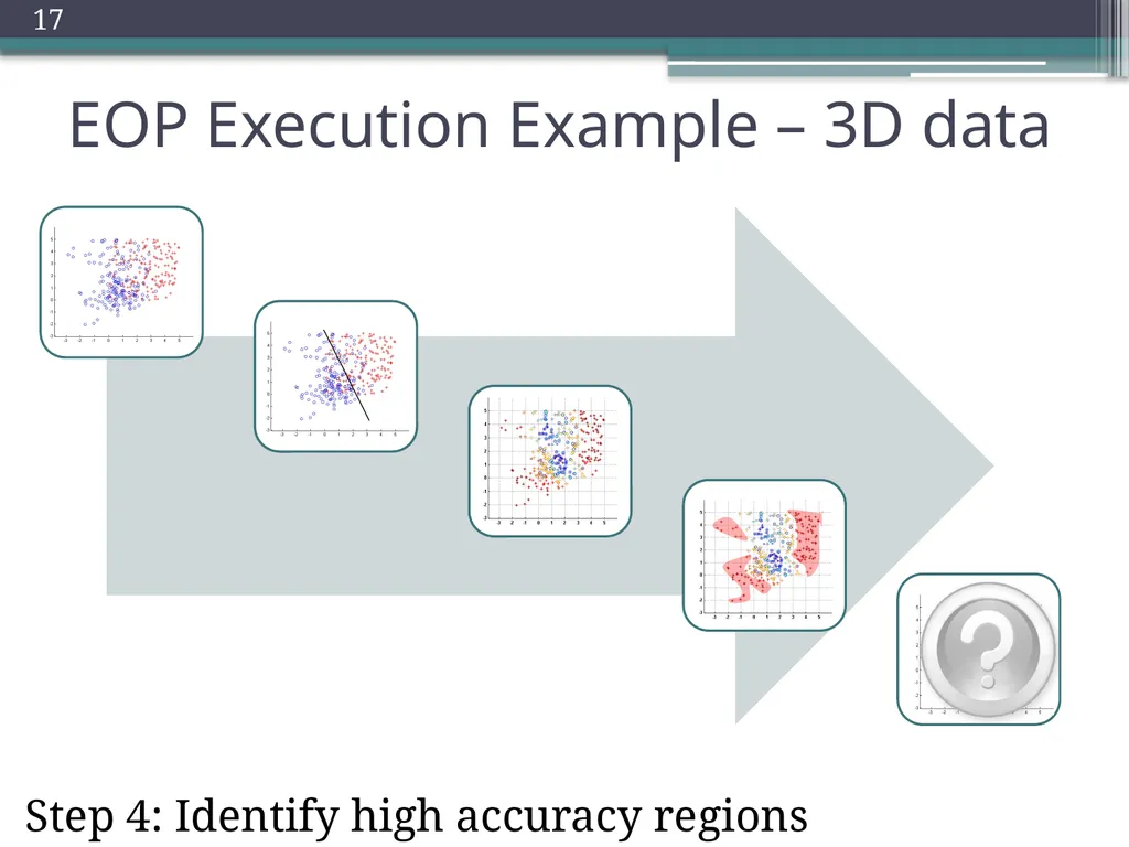
slide17. Step 4: Identify high accuracy regions 17 EOP Execution Example – 3D data<br>
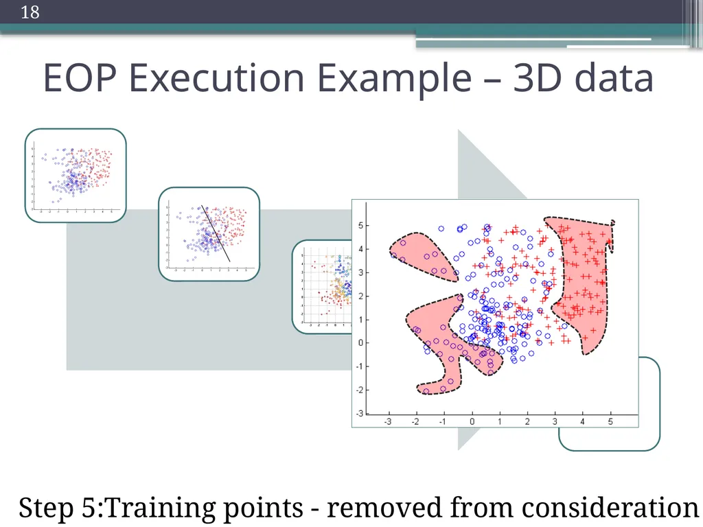
slide18. Step 5:Training points - removed from consideration 18 EOP Execution Example – 3D data<br>
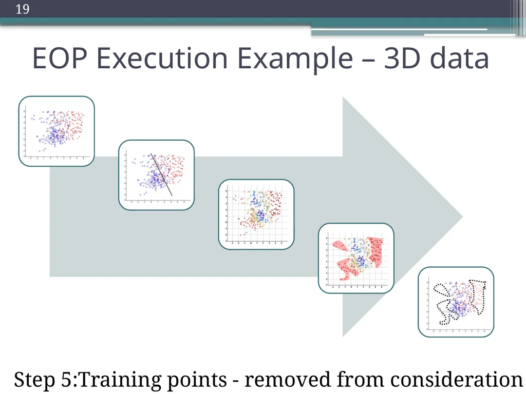
slide19. 19 Step 5:Training points - removed from consideration EOP Execution Example – 3D data<br>
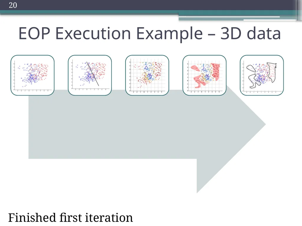
slide20. Finished first iteration 20 EOP Execution Example – 3D data<br>
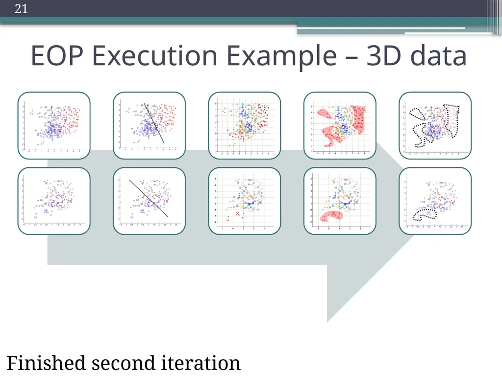
slide21. 21 EOP Execution Example – 3D data Finished second iteration<br>
slide22. Iterate until all data is accounted for
or error cannot be decreased 22 EOP Execution Example – 3D data<br>
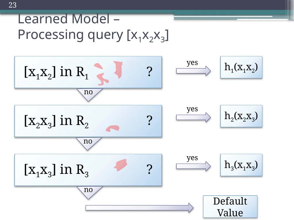
slide23. Learned Model – Processing query [x1x2x3] [x1x2] in R1 ? [x2x3] in R2 ? [x1x3] in R3 ? h1(x1x2) h2(x2x3) h3(x1x3) Default Value yes yes yes no no no 23<br>
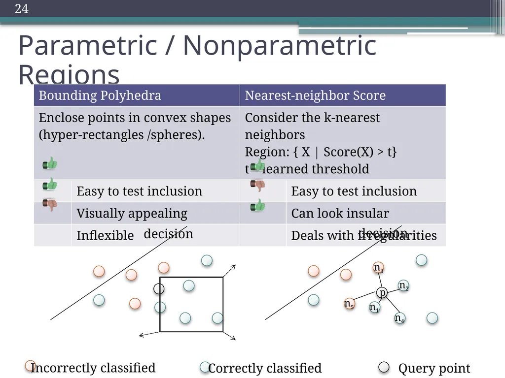
slide24. Parametric / Nonparametric Regions 24<br>
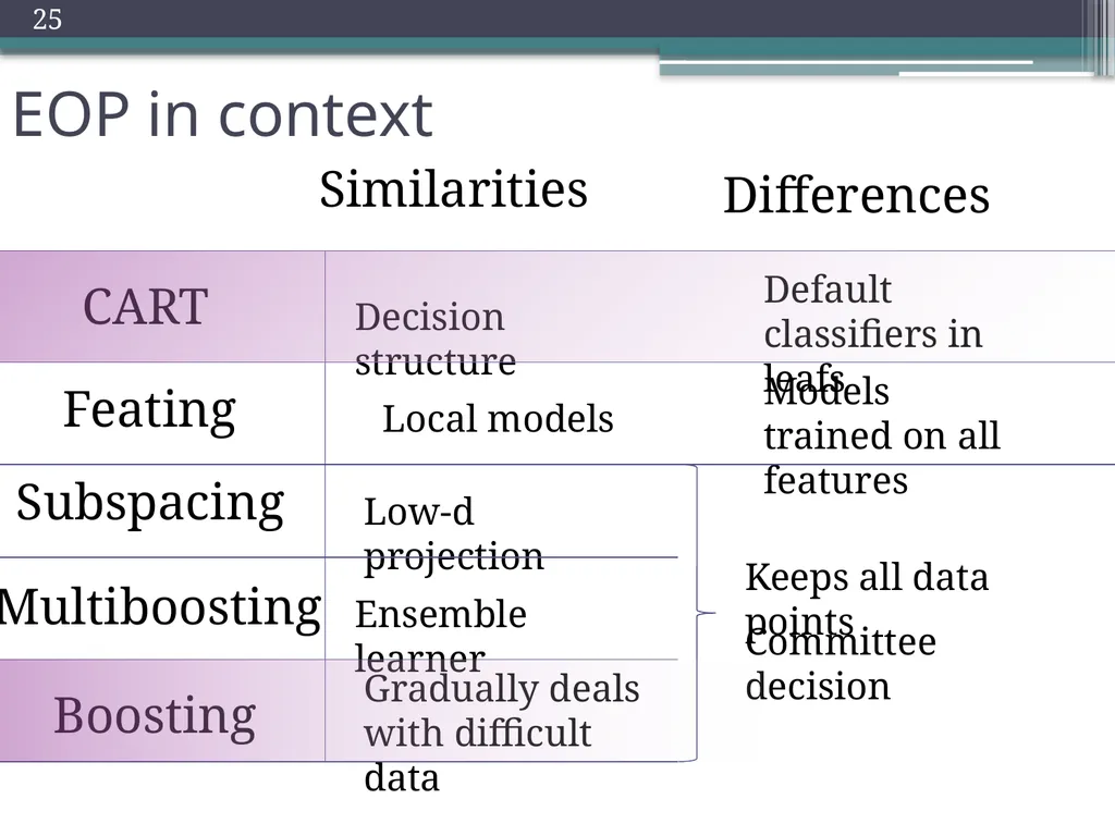
slide25. EOP in context Local models Models trained on all features Feating 25 Similarities Differences CART Decision structure Default classifiers in leafs Subspacing Low-d projection Keeps all data points Boosting Multiboosting Committee decision Gradually deals with difficult data Ensemble learner<br>
slide26. Outline Motivation: need for interpretable models
Overview of data analysis tools
Model evaluation – accuracy vs complexity
Model evaluation – understandability
Example applications
Summary 26<br>
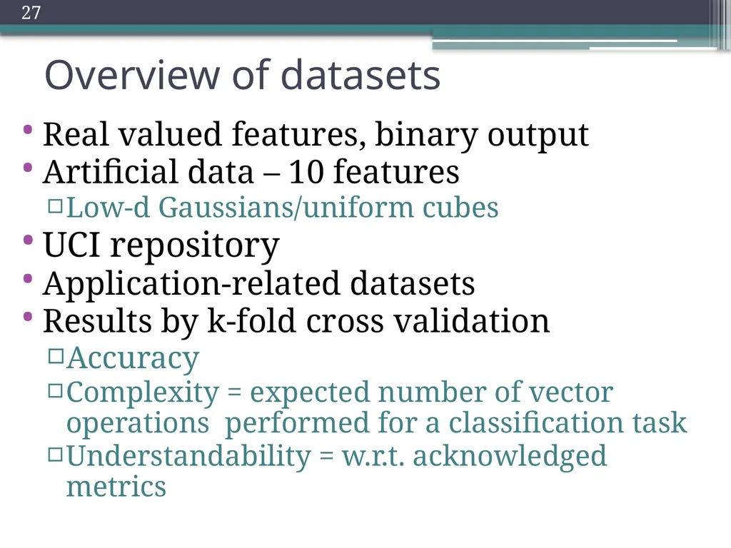
slide27. Overview of datasets Real valued features, binary output
Artificial data – 10 features
Low-d Gaussians/uniform cubes
UCI repository
Application-related datasets
Results by k-fold cross validation
Accuracy
Complexity = expected number of vector operations performed for a classification task
Understandability = w.r.t. acknowledged metrics 27<br>
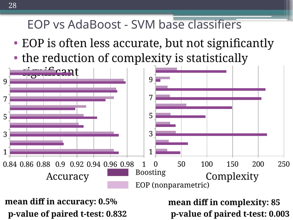
slide28. EOP vs AdaBoost - SVM base classifiers EOP is often less accurate, but not significantly
the reduction of complexity is statistically significant p-value of paired t-test: 0.832 p-value of paired t-test: 0.003 Accuracy Complexity 28 mean diff in accuracy: 0.5% mean diff in complexity: 85<br>
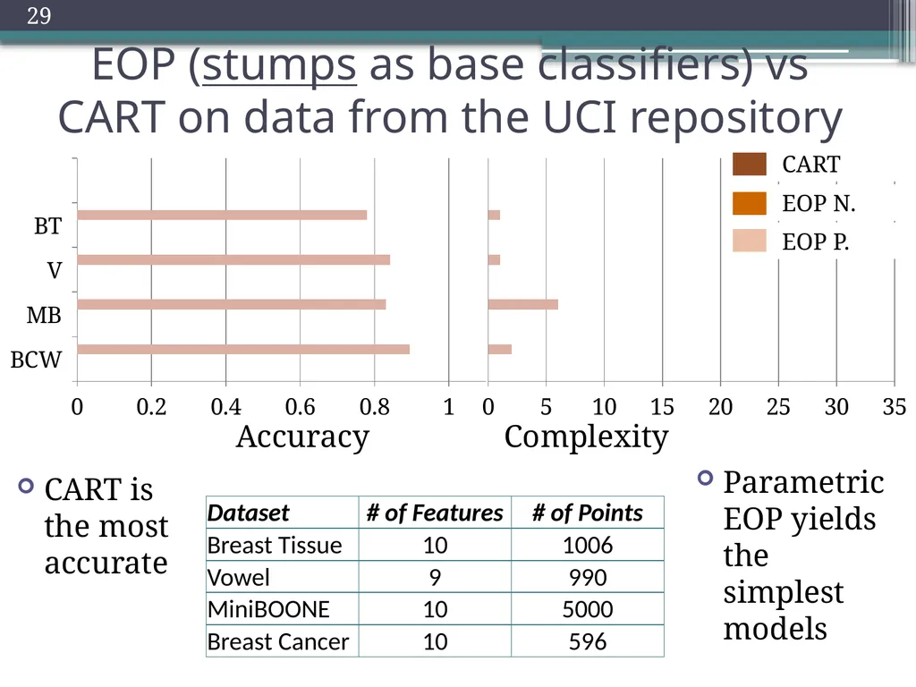
slide29. EOP (stumps as base classifiers) vs CART on data from the UCI repository Accuracy Complexity EOP P. 29 CART is the most accurate Parametric EOP yields the simplest models<br>
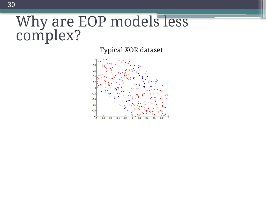
slide30. Typical XOR dataset 30 Why are EOP models less complex?<br>
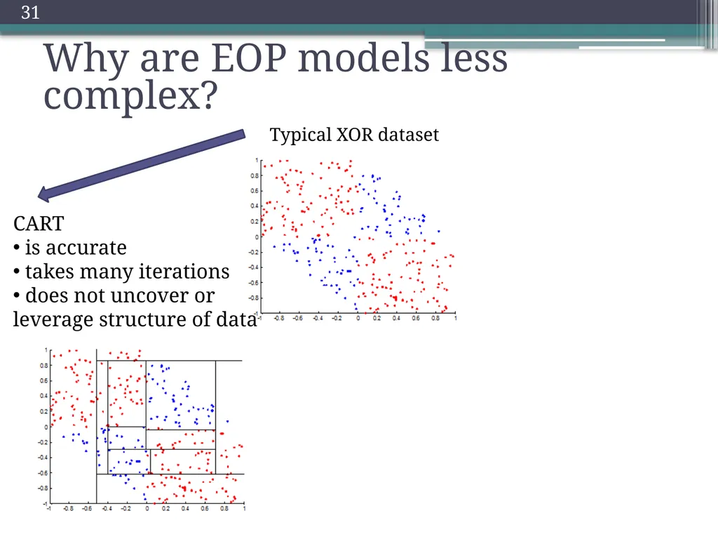
slide31. Typical XOR dataset 31 Why are EOP models less complex?<br>
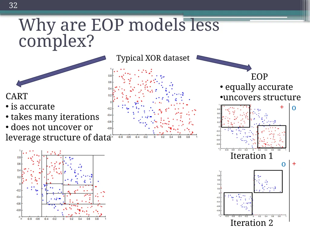
slide32. Typical XOR dataset EOP
equally accurate
uncovers structure Iteration 1 Iteration 2 32 + o o + Why are EOP models less complex?<br>
slide33. At low complexities, EOP is typically more accurate Error Variation With Model Complexity for EOP and CART Depth of decision tree/list Error 33<br>
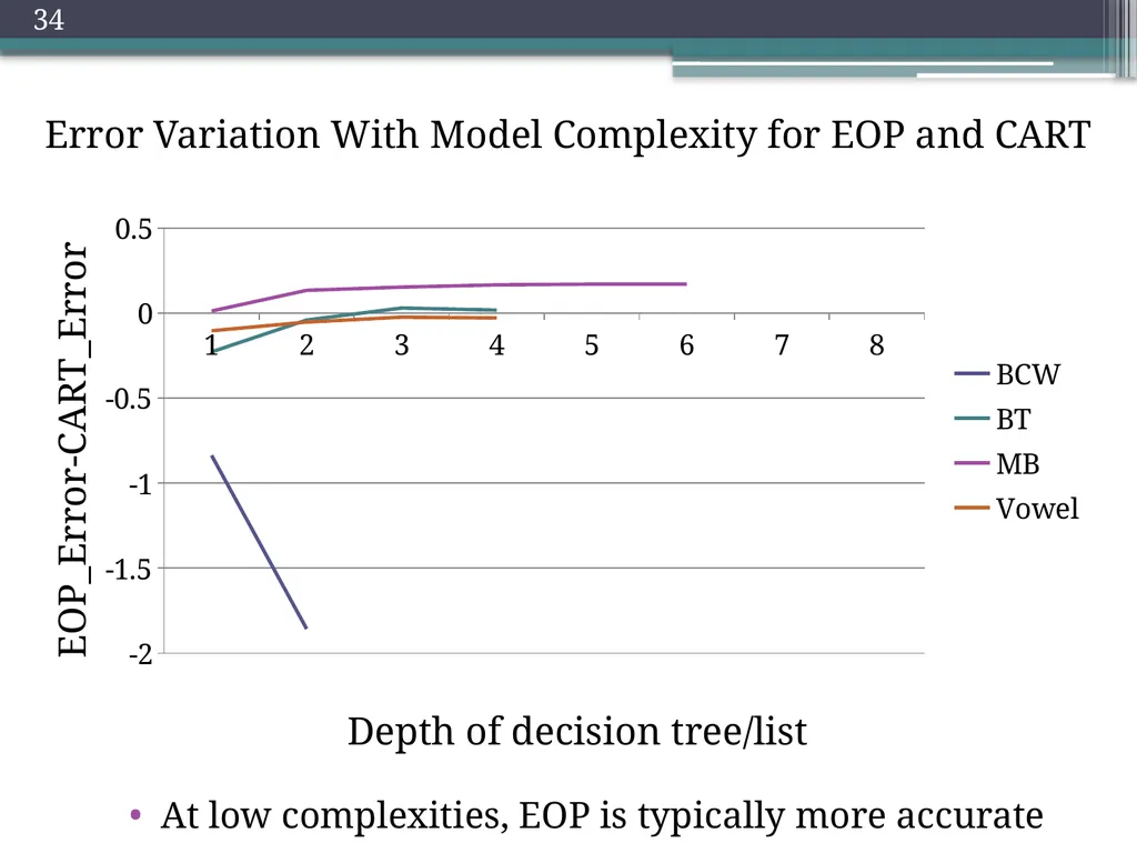
slide34. At low complexities, EOP is typically more accurate Error Variation With Model Complexity for EOP and CART Depth of decision tree/list EOP_Error-CART_Error 34<br>
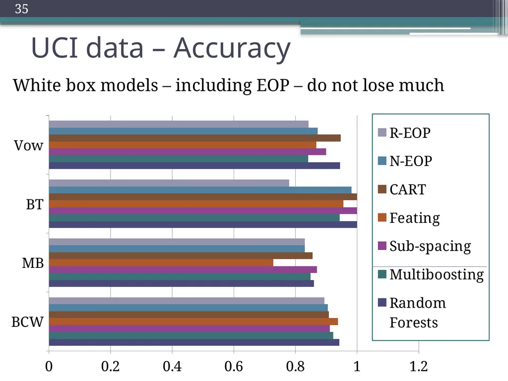
slide35. UCI data – Accuracy 35 White box models – including EOP – do not lose much<br>
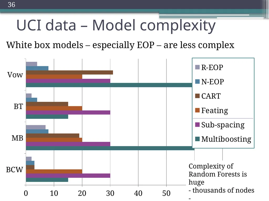
slide36. UCI data – Model complexity 36 Complexity of Random Forests is huge
- thousands of nodes - White box models – especially EOP – are less complex<br>
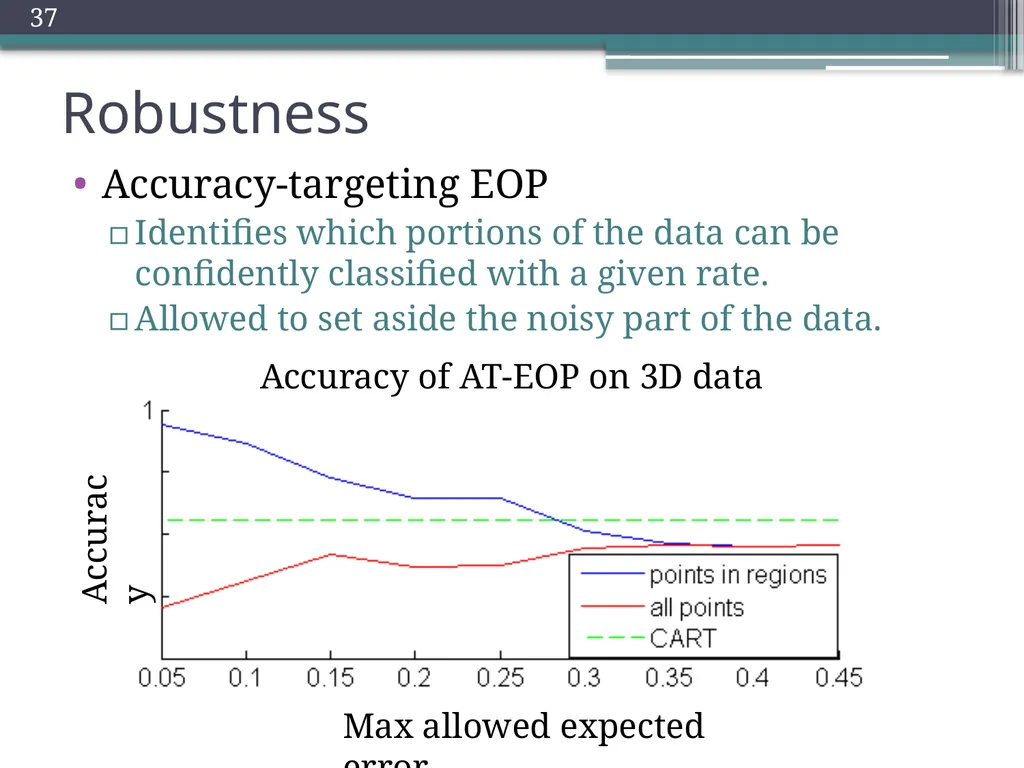
slide37. Robustness Accuracy-targeting EOP
Identifies which portions of the data can be confidently classified with a given rate.
Allowed to set aside the noisy part of the data. 37<br>
slide38. Outline Motivation: need for interpretable models
Overview of data analysis tools
Model evaluation – accuracy vs complexity
Model evaluation – understandability
Example applications
Summary 38<br>
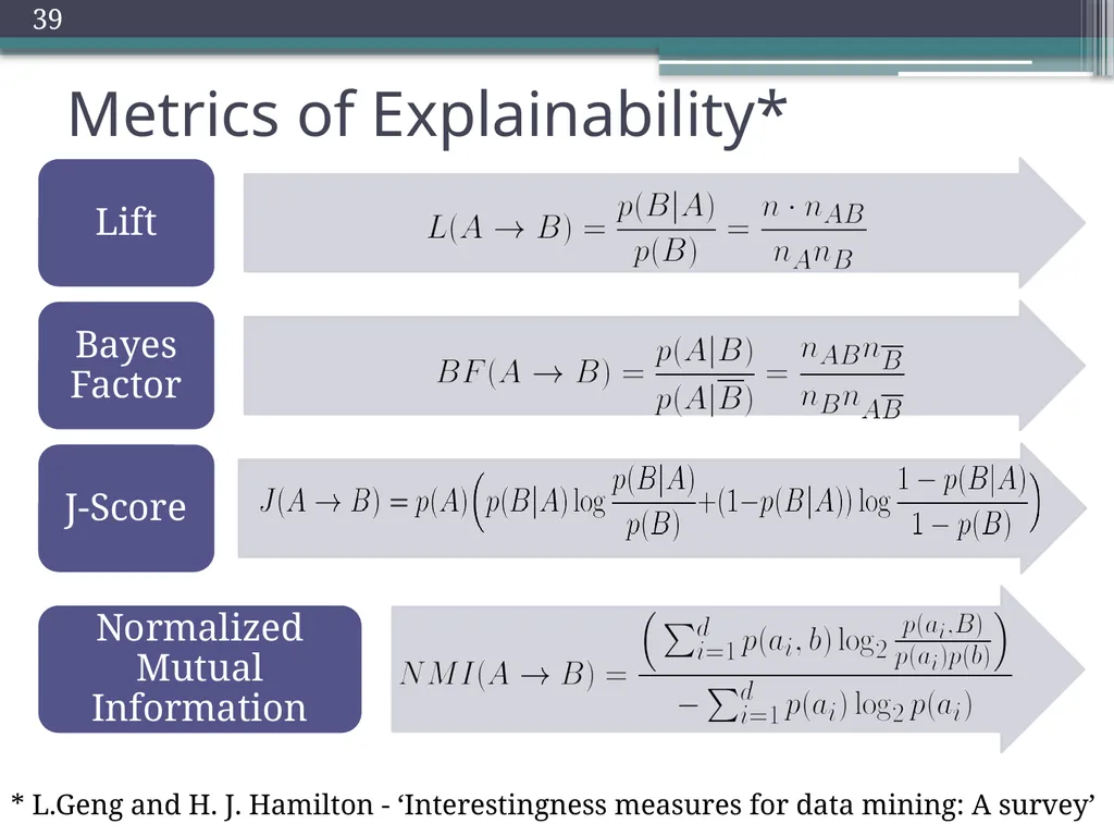
slide39. Metrics of Explainability* 39 * L.Geng and H. J. Hamilton - ‘Interestingness measures for data mining: A survey’<br>
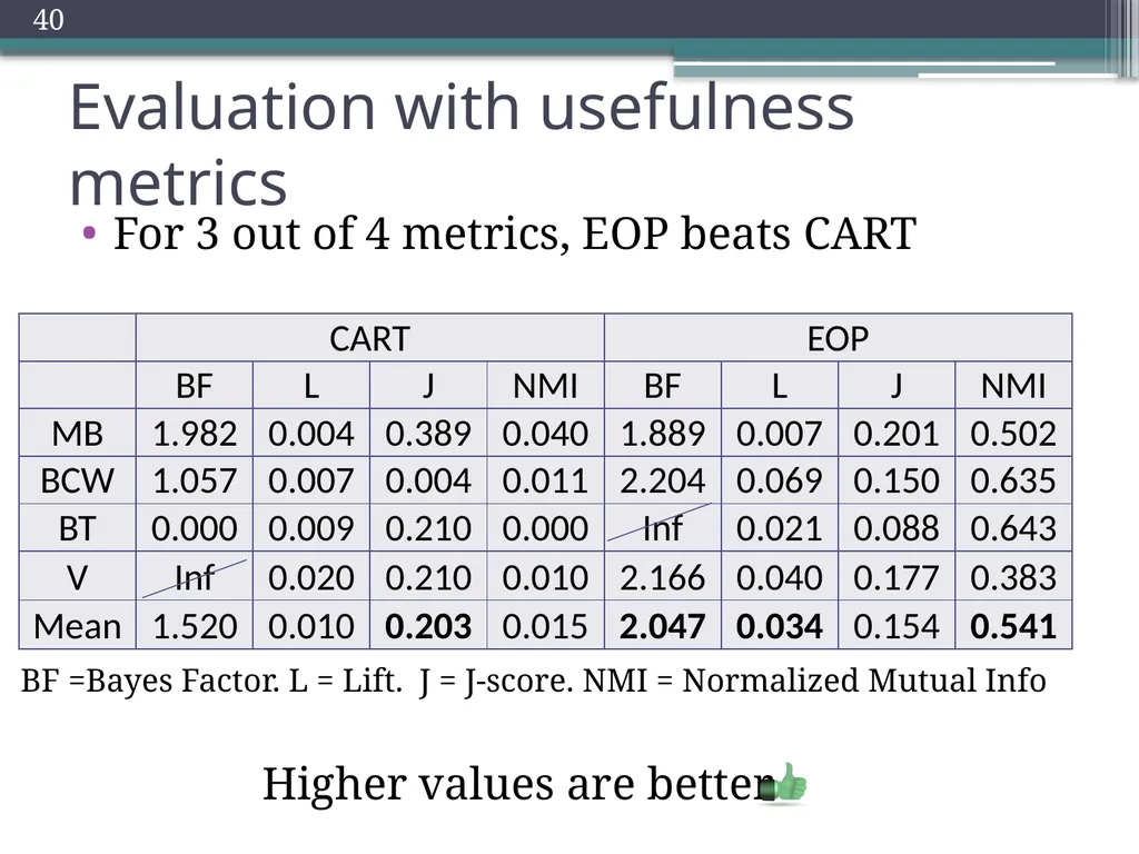
slide40. Evaluation with usefulness metrics For 3 out of 4 metrics, EOP beats CART BF =Bayes Factor. L = Lift. J = J-score. NMI = Normalized Mutual Info 40 Higher values are better<br>
slide41. Outline Motivation: need for interpretable models
Overview of data analysis tools
Model evaluation – accuracy vs complexity
Model evaluation – understandability
Example applications
Summary 41<br>
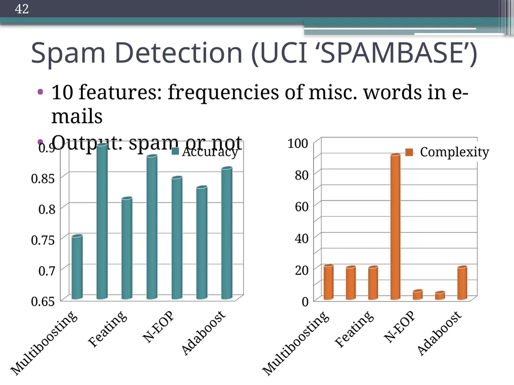
slide42. Spam Detection (UCI ‘SPAMBASE’) 10 features: frequencies of misc. words in e-mails
Output: spam or not 42 Complexity<br>
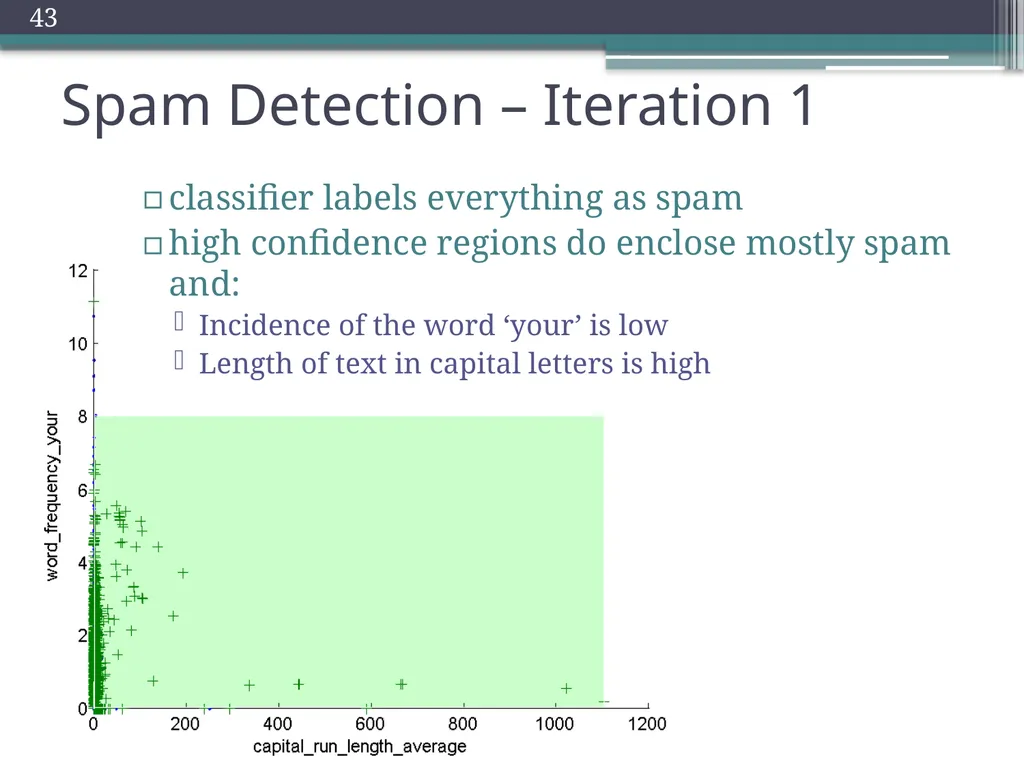
slide43. Spam Detection – Iteration 1 classifier labels everything as spam
high confidence regions do enclose mostly spam and:
Incidence of the word ‘your’ is low
Length of text in capital letters is high 43<br>
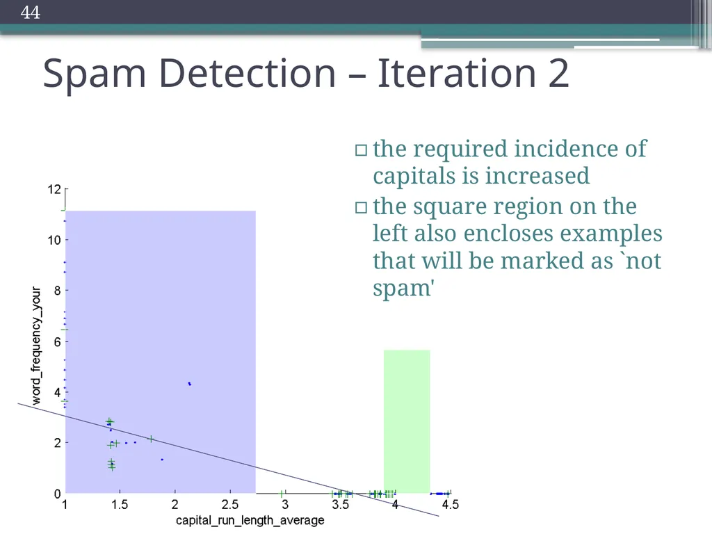
slide44. Spam Detection – Iteration 2 the required incidence of capitals is increased
the square region on the left also encloses examples that will be marked as `not spam' 44<br>
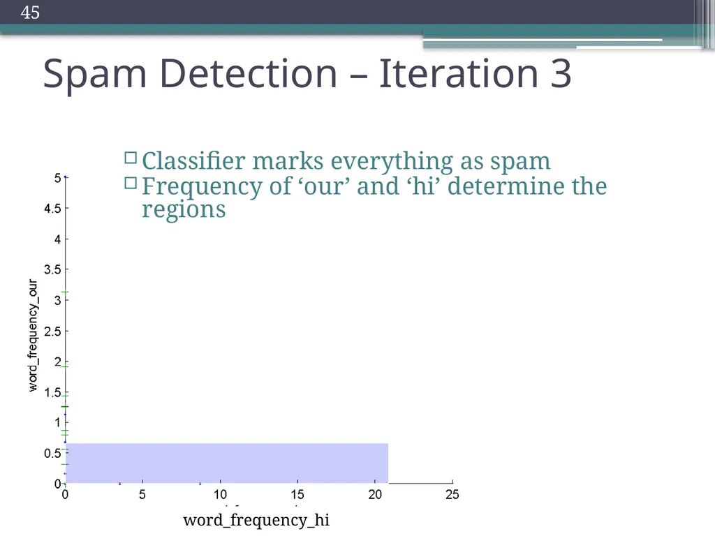
slide45. Spam Detection – Iteration 3 45 Classifier marks everything as spam
Frequency of ‘our’ and ‘hi’ determine the regions<br>
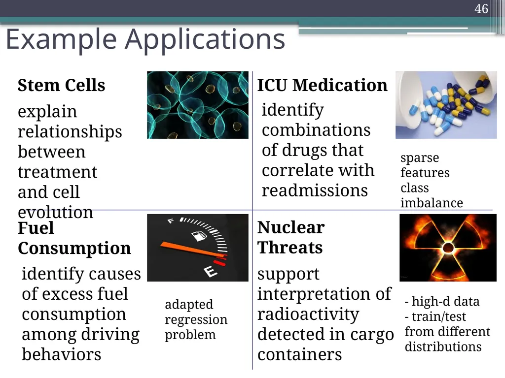
slide46. Example Applications 46 Stem Cells ICU Medication Fuel Consumption Nuclear Threats explain relationships between treatment
and cell evolution identify combinations of drugs that correlate with readmissions identify causes of excess fuel consumption among driving behaviors support interpretation of radioactivity detected in cargo containers sparse features
class imbalance - high-d data
- train/test from different distributions adapted regression problem<br>
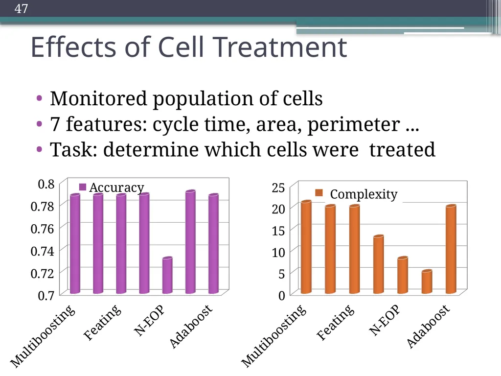
slide47. Effects of Cell Treatment Monitored population of cells
7 features: cycle time, area, perimeter ...
Task: determine which cells were treated 47 Complexity<br>
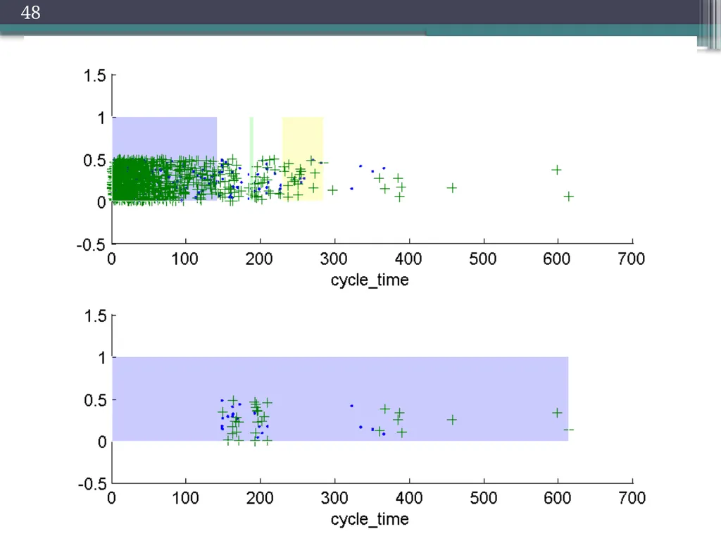
slide48. 48<br>
slide49. Mimic Medication Data Information about administered medication
Features: dosage for each drug
Task: predict patient return to ICU 49 Complexity<br>
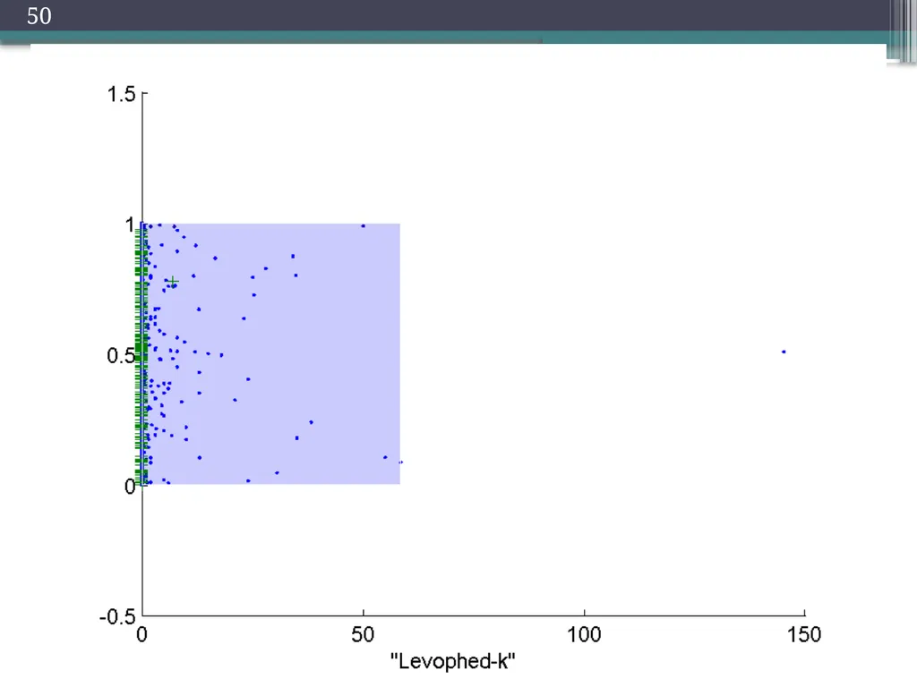
slide50. 50<br>
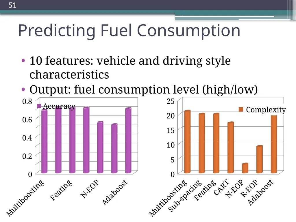
slide51. Predicting Fuel Consumption 10 features: vehicle and driving style characteristics
Output: fuel consumption level (high/low) 51 Complexity<br>
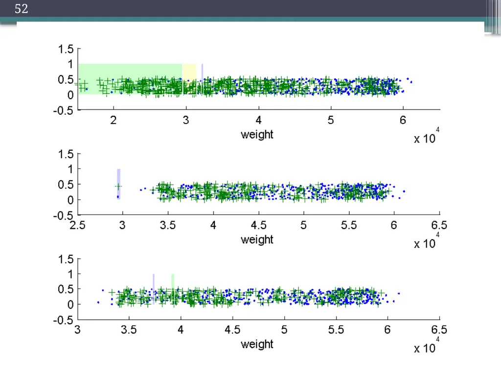
slide52. 52<br>
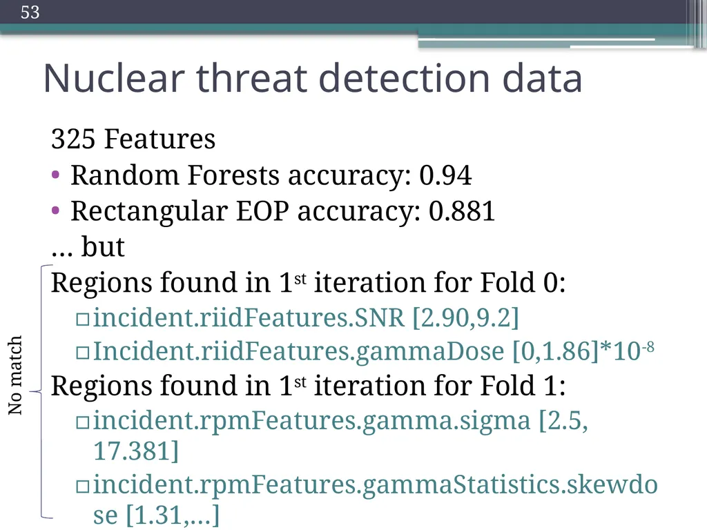
slide53. Nuclear threat detection data 325 Features
Random Forests accuracy: 0.94
Rectangular EOP accuracy: 0.881
… but
Regions found in 1st iteration for Fold 0:
incident.riidFeatures.SNR [2.90,9.2]
Incident.riidFeatures.gammaDose [0,1.86]*10-8
Regions found in 1st iteration for Fold 1:
incident.rpmFeatures.gamma.sigma [2.5, 17.381]
incident.rpmFeatures.gammaStatistics.skewdose [1.31,…] No match 53<br>
slide54. Feating and EOP Decision Structures to pick right classification model Flexible Regions Tiles in feature space Decision Tree Decision List Models trained on all features Models trained on subspaces EOP Feating 54<br>
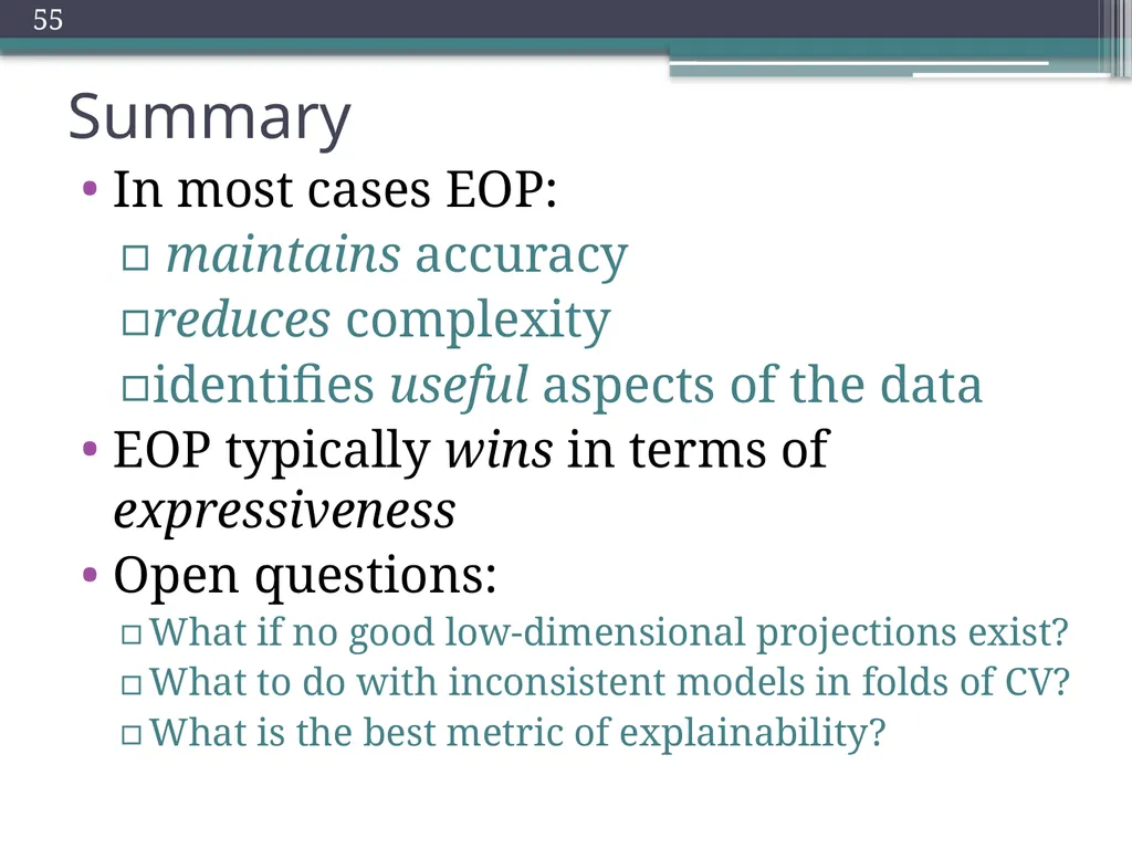
slide55. Summary In most cases EOP:
maintains accuracy
reduces complexity
identifies useful aspects of the data
EOP typically wins in terms of expressiveness
Open questions:
What if no good low-dimensional projections exist?
What to do with inconsistent models in folds of CV?
What is the best metric of explainability? 55<br>
Madalina Fiterau 22nd of February 2012 1<br>
slide2. Outline Motivation: need for interpretable models
Overview of data analysis tools
Model evaluation – accuracy vs complexity
Model evaluation – understandability
Example applications
Summary 2<br>
slide3. Example Application: Nuclear Threat Detection Border control: vehicles are scanned
Human in the loop interpreting results vehicle scan prediction feedback 3<br>
slide4. Boosted Decision Stumps Accurate, but hard to interpret How is the prediction derived from the input? 4<br>
slide5. Decision Tree – More Interpretable Radiation > x% Payload type = ceramics Uranium level > max. admissible for ceramics Consider balance of Th232, Ra226 and Co60 Clear yes no yes no Threat yes no 5<br>
slide6. Motivation 6 Many users are willing to trade accuracy to
better understand the system-yielded results
Need: simple, interpretable model
Need: explanatory prediction process<br>
slide7. Analysis Tools – Black-box 7<br>
slide8. Analysis Tools – White-box 8<br>
slide9. Explanation-Oriented Partitioning (X,Y) plot 9<br>
slide10. EOP Execution Example – 3D data Step 1: Select a projection - (X1,X2) 10<br>
slide11. Step 1: Select a projection - (X1,X2) 11 EOP Execution Example – 3D data<br>
slide12. Step 2: Choose a good classifier - call it h1 h1 12 EOP Execution Example – 3D data<br>
slide13. Step 2: Choose a good classifier - call it h1 13 EOP Execution Example – 3D data<br>
slide14. Step 3: Estimate accuracy of h1 at each point 14 EOP Execution Example – 3D data<br>
slide15. Step 3: Estimate accuracy of h1 for each point 15 EOP Execution Example – 3D data<br>
slide16. Step 4: Identify high accuracy regions 16 EOP Execution Example – 3D data<br>
slide17. Step 4: Identify high accuracy regions 17 EOP Execution Example – 3D data<br>
slide18. Step 5:Training points - removed from consideration 18 EOP Execution Example – 3D data<br>
slide19. 19 Step 5:Training points - removed from consideration EOP Execution Example – 3D data<br>
slide20. Finished first iteration 20 EOP Execution Example – 3D data<br>
slide21. 21 EOP Execution Example – 3D data Finished second iteration<br>
slide22. Iterate until all data is accounted for
or error cannot be decreased 22 EOP Execution Example – 3D data<br>
slide23. Learned Model – Processing query [x1x2x3] [x1x2] in R1 ? [x2x3] in R2 ? [x1x3] in R3 ? h1(x1x2) h2(x2x3) h3(x1x3) Default Value yes yes yes no no no 23<br>
slide24. Parametric / Nonparametric Regions 24<br>
slide25. EOP in context Local models Models trained on all features Feating 25 Similarities Differences CART Decision structure Default classifiers in leafs Subspacing Low-d projection Keeps all data points Boosting Multiboosting Committee decision Gradually deals with difficult data Ensemble learner<br>
slide26. Outline Motivation: need for interpretable models
Overview of data analysis tools
Model evaluation – accuracy vs complexity
Model evaluation – understandability
Example applications
Summary 26<br>
slide27. Overview of datasets Real valued features, binary output
Artificial data – 10 features
Low-d Gaussians/uniform cubes
UCI repository
Application-related datasets
Results by k-fold cross validation
Accuracy
Complexity = expected number of vector operations performed for a classification task
Understandability = w.r.t. acknowledged metrics 27<br>
slide28. EOP vs AdaBoost - SVM base classifiers EOP is often less accurate, but not significantly
the reduction of complexity is statistically significant p-value of paired t-test: 0.832 p-value of paired t-test: 0.003 Accuracy Complexity 28 mean diff in accuracy: 0.5% mean diff in complexity: 85<br>
slide29. EOP (stumps as base classifiers) vs CART on data from the UCI repository Accuracy Complexity EOP P. 29 CART is the most accurate Parametric EOP yields the simplest models<br>
slide30. Typical XOR dataset 30 Why are EOP models less complex?<br>
slide31. Typical XOR dataset 31 Why are EOP models less complex?<br>
slide32. Typical XOR dataset EOP
equally accurate
uncovers structure Iteration 1 Iteration 2 32 + o o + Why are EOP models less complex?<br>
slide33. At low complexities, EOP is typically more accurate Error Variation With Model Complexity for EOP and CART Depth of decision tree/list Error 33<br>
slide34. At low complexities, EOP is typically more accurate Error Variation With Model Complexity for EOP and CART Depth of decision tree/list EOP_Error-CART_Error 34<br>
slide35. UCI data – Accuracy 35 White box models – including EOP – do not lose much<br>
slide36. UCI data – Model complexity 36 Complexity of Random Forests is huge
- thousands of nodes - White box models – especially EOP – are less complex<br>
slide37. Robustness Accuracy-targeting EOP
Identifies which portions of the data can be confidently classified with a given rate.
Allowed to set aside the noisy part of the data. 37<br>
slide38. Outline Motivation: need for interpretable models
Overview of data analysis tools
Model evaluation – accuracy vs complexity
Model evaluation – understandability
Example applications
Summary 38<br>
slide39. Metrics of Explainability* 39 * L.Geng and H. J. Hamilton - ‘Interestingness measures for data mining: A survey’<br>
slide40. Evaluation with usefulness metrics For 3 out of 4 metrics, EOP beats CART BF =Bayes Factor. L = Lift. J = J-score. NMI = Normalized Mutual Info 40 Higher values are better<br>
slide41. Outline Motivation: need for interpretable models
Overview of data analysis tools
Model evaluation – accuracy vs complexity
Model evaluation – understandability
Example applications
Summary 41<br>
slide42. Spam Detection (UCI ‘SPAMBASE’) 10 features: frequencies of misc. words in e-mails
Output: spam or not 42 Complexity<br>
slide43. Spam Detection – Iteration 1 classifier labels everything as spam
high confidence regions do enclose mostly spam and:
Incidence of the word ‘your’ is low
Length of text in capital letters is high 43<br>
slide44. Spam Detection – Iteration 2 the required incidence of capitals is increased
the square region on the left also encloses examples that will be marked as `not spam' 44<br>
slide45. Spam Detection – Iteration 3 45 Classifier marks everything as spam
Frequency of ‘our’ and ‘hi’ determine the regions<br>
slide46. Example Applications 46 Stem Cells ICU Medication Fuel Consumption Nuclear Threats explain relationships between treatment
and cell evolution identify combinations of drugs that correlate with readmissions identify causes of excess fuel consumption among driving behaviors support interpretation of radioactivity detected in cargo containers sparse features
class imbalance - high-d data
- train/test from different distributions adapted regression problem<br>
slide47. Effects of Cell Treatment Monitored population of cells
7 features: cycle time, area, perimeter ...
Task: determine which cells were treated 47 Complexity<br>
slide48. 48<br>
slide49. Mimic Medication Data Information about administered medication
Features: dosage for each drug
Task: predict patient return to ICU 49 Complexity<br>
slide50. 50<br>
slide51. Predicting Fuel Consumption 10 features: vehicle and driving style characteristics
Output: fuel consumption level (high/low) 51 Complexity<br>
slide52. 52<br>
slide53. Nuclear threat detection data 325 Features
Random Forests accuracy: 0.94
Rectangular EOP accuracy: 0.881
… but
Regions found in 1st iteration for Fold 0:
incident.riidFeatures.SNR [2.90,9.2]
Incident.riidFeatures.gammaDose [0,1.86]*10-8
Regions found in 1st iteration for Fold 1:
incident.rpmFeatures.gamma.sigma [2.5, 17.381]
incident.rpmFeatures.gammaStatistics.skewdose [1.31,…] No match 53<br>
slide54. Feating and EOP Decision Structures to pick right classification model Flexible Regions Tiles in feature space Decision Tree Decision List Models trained on all features Models trained on subspaces EOP Feating 54<br>
slide55. Summary In most cases EOP:
maintains accuracy
reduces complexity
identifies useful aspects of the data
EOP typically wins in terms of expressiveness
Open questions:
What if no good low-dimensional projections exist?
What to do with inconsistent models in folds of CV?
What is the best metric of explainability? 55<br>