
Understanding Large Language Models A Natural
DP
Published · 74 slides · 0 views
1 / 1
Description
Understanding Large Language Models A Natural Language Processing Lecture Omkar Brahmbhatt tuu62443temple.edu MS Computer Science student Darlin Kola tun32955temple.edu MS Computer Science student Varshil Patel tuu73592temple.edu MS
Related Topics
Share
Embed code
Download this presentation From Below
"Understanding Large Language Models A Natural" is the property of its rightful owner. Permission is granted to download and print the materials on this website for personal, non-commercial use only, and to display it on your personal computer provided you do not modify the materials and that you retain all copyright notices contained in the materials. By downloading content from our website, you accept the terms of this agreement.
Presentation Transcript
01
Understanding Large Language Models A Natural Language Processing Lecture Omkar Brahmbhatt
tuu62443@temple.edu MS Computer Science student Darlin Kola
tun32955@temple.edu MS Computer Science student Varshil Patel
tuu73592@temple.edu MS Computer Science student CIS 5543: COMPUTER VISION Spring 2026<br>
tuu62443@temple.edu MS Computer Science student Darlin Kola
tun32955@temple.edu MS Computer Science student Varshil Patel
tuu73592@temple.edu MS Computer Science student CIS 5543: COMPUTER VISION Spring 2026<br>
02
Part 1:
How LLMs Work: The Power of Token Prediction From Text to Probabilities<br>
How LLMs Work: The Power of Token Prediction From Text to Probabilities<br>
03
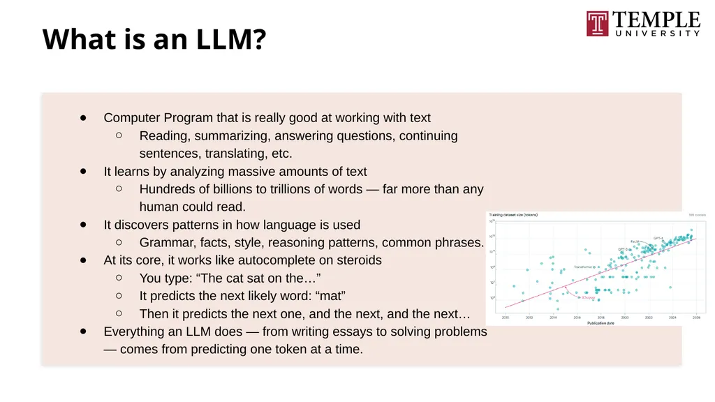
What is an LLM? Computer Program that is really good at working with text
Reading, summarizing, answering questions, continuing sentences, translating, etc.
It learns by analyzing massive amounts of text
Hundreds of billions to trillions of words — far more than any human could read.
It discovers patterns in how language is used
Grammar, facts, style, reasoning patterns, common phrases.
At its core, it works like autocomplete on steroids
You type: “The cat sat on the…”
It predicts the next likely word: “mat”
Then it predicts the next one, and the next, and the next…
Everything an LLM does — from writing essays to solving problems — comes from predicting one token at a time.<br>
Reading, summarizing, answering questions, continuing sentences, translating, etc.
It learns by analyzing massive amounts of text
Hundreds of billions to trillions of words — far more than any human could read.
It discovers patterns in how language is used
Grammar, facts, style, reasoning patterns, common phrases.
At its core, it works like autocomplete on steroids
You type: “The cat sat on the…”
It predicts the next likely word: “mat”
Then it predicts the next one, and the next, and the next…
Everything an LLM does — from writing essays to solving problems — comes from predicting one token at a time.<br>
04
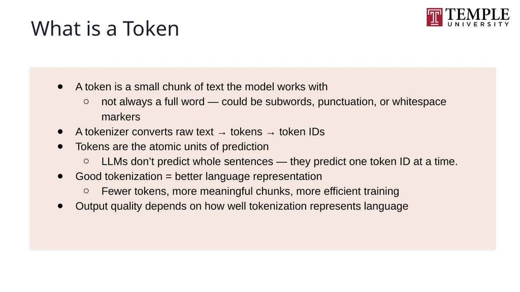
What is a Token A token is a small chunk of text the model works with
not always a full word — could be subwords, punctuation, or whitespace markers
A tokenizer converts raw text → tokens → token IDs
Tokens are the atomic units of prediction
LLMs don’t predict whole sentences — they predict one token ID at a time.
Good tokenization = better language representation
Fewer tokens, more meaningful chunks, more efficient training
Output quality depends on how well tokenization represents language<br>
not always a full word — could be subwords, punctuation, or whitespace markers
A tokenizer converts raw text → tokens → token IDs
Tokens are the atomic units of prediction
LLMs don’t predict whole sentences — they predict one token ID at a time.
Good tokenization = better language representation
Fewer tokens, more meaningful chunks, more efficient training
Output quality depends on how well tokenization represents language<br>
05
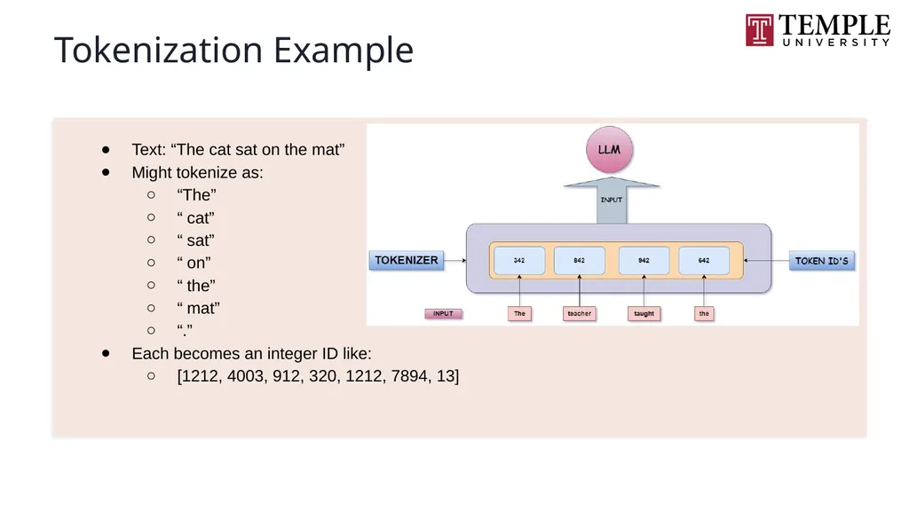
Tokenization Example Text: “The cat sat on the mat”
Might tokenize as:
“The”
“ cat”
“ sat”
“ on”
“ the”
“ mat”
“.”
Each becomes an integer ID like:
[1212, 4003, 912, 320, 1212, 7894, 13]<br>
Might tokenize as:
“The”
“ cat”
“ sat”
“ on”
“ the”
“ mat”
“.”
Each becomes an integer ID like:
[1212, 4003, 912, 320, 1212, 7894, 13]<br>
06
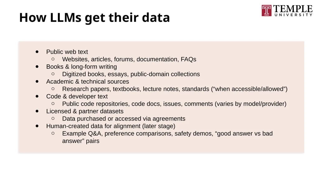
How LLMs get their data Public web text
Websites, articles, forums, documentation, FAQs
Books & long-form writing
Digitized books, essays, public-domain collections
Academic & technical sources
Research papers, textbooks, lecture notes, standards (“when accessible/allowed”)
Code & developer text
Public code repositories, code docs, issues, comments (varies by model/provider)
Licensed & partner datasets
Data purchased or accessed via agreements
Human-created data for alignment (later stage)
Example Q&A, preference comparisons, safety demos, “good answer vs bad answer” pairs<br>
Websites, articles, forums, documentation, FAQs
Books & long-form writing
Digitized books, essays, public-domain collections
Academic & technical sources
Research papers, textbooks, lecture notes, standards (“when accessible/allowed”)
Code & developer text
Public code repositories, code docs, issues, comments (varies by model/provider)
Licensed & partner datasets
Data purchased or accessed via agreements
Human-created data for alignment (later stage)
Example Q&A, preference comparisons, safety demos, “good answer vs bad answer” pairs<br>
07
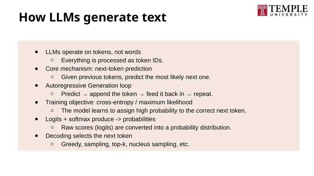
How LLMs generate text LLMs operate on tokens, not words
Everything is processed as token IDs.
Core mechanism: next-token prediction
Given previous tokens, predict the most likely next one.
Autoregressive Generation loop
Predict → append the token → feed it back in → repeat.
Training objective: cross‑entropy / maximum likelihood
The model learns to assign high probability to the correct next token.
Logits + softmax produce -> probabilities
Raw scores (logits) are converted into a probability distribution.
Decoding selects the next token
Greedy, sampling, top‑k, nucleus sampling, etc.<br>
Everything is processed as token IDs.
Core mechanism: next-token prediction
Given previous tokens, predict the most likely next one.
Autoregressive Generation loop
Predict → append the token → feed it back in → repeat.
Training objective: cross‑entropy / maximum likelihood
The model learns to assign high probability to the correct next token.
Logits + softmax produce -> probabilities
Raw scores (logits) are converted into a probability distribution.
Decoding selects the next token
Greedy, sampling, top‑k, nucleus sampling, etc.<br>
08
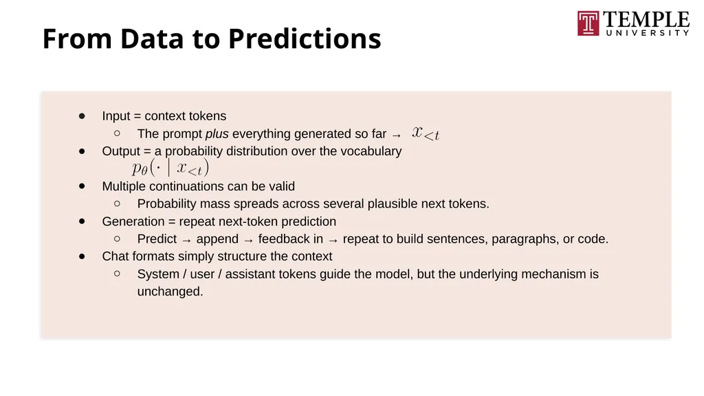
From Data to Predictions Input = context tokens
The prompt plus everything generated so far →
Output = a probability distribution over the vocabulary
Multiple continuations can be valid
Probability mass spreads across several plausible next tokens.
Generation = repeat next‑token prediction
Predict → append → feedback in → repeat to build sentences, paragraphs, or code.
Chat formats simply structure the context
System / user / assistant tokens guide the model, but the underlying mechanism is unchanged.<br>
The prompt plus everything generated so far →
Output = a probability distribution over the vocabulary
Multiple continuations can be valid
Probability mass spreads across several plausible next tokens.
Generation = repeat next‑token prediction
Predict → append → feedback in → repeat to build sentences, paragraphs, or code.
Chat formats simply structure the context
System / user / assistant tokens guide the model, but the underlying mechanism is unchanged.<br>
09
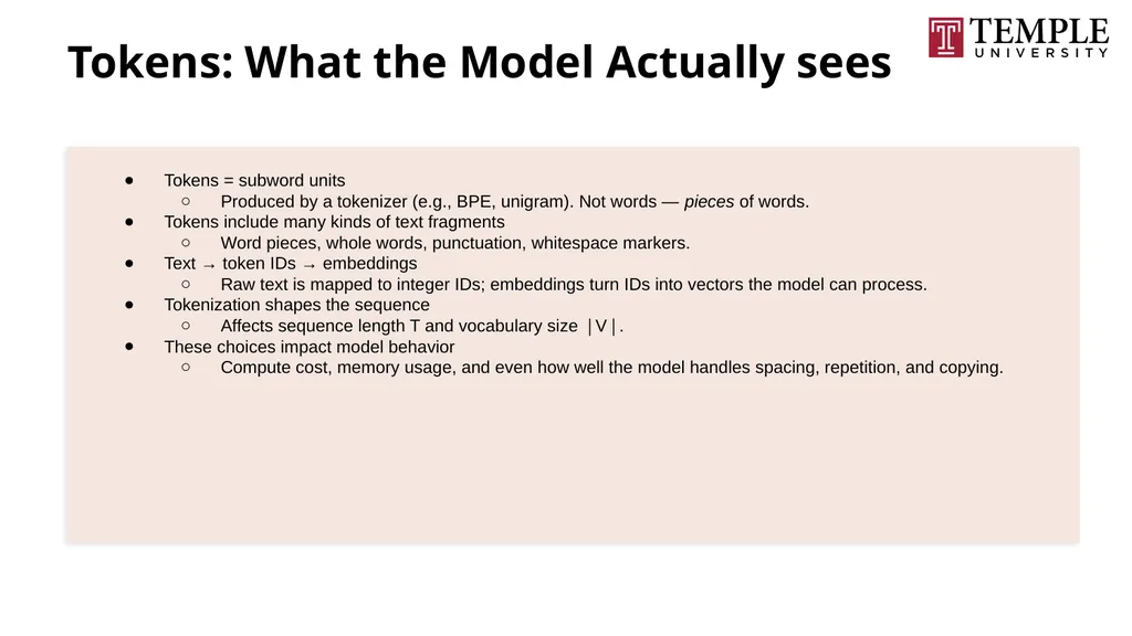
Tokens: What the Model Actually sees Tokens = subword units
Produced by a tokenizer (e.g., BPE, unigram). Not words — pieces of words.
Tokens include many kinds of text fragments
Word pieces, whole words, punctuation, whitespace markers.
Text → token IDs → embeddings
Raw text is mapped to integer IDs; embeddings turn IDs into vectors the model can process.
Tokenization shapes the sequence
Affects sequence length T and vocabulary size ∣V∣.
These choices impact model behavior
Compute cost, memory usage, and even how well the model handles spacing, repetition, and copying.<br>
Produced by a tokenizer (e.g., BPE, unigram). Not words — pieces of words.
Tokens include many kinds of text fragments
Word pieces, whole words, punctuation, whitespace markers.
Text → token IDs → embeddings
Raw text is mapped to integer IDs; embeddings turn IDs into vectors the model can process.
Tokenization shapes the sequence
Affects sequence length T and vocabulary size ∣V∣.
These choices impact model behavior
Compute cost, memory usage, and even how well the model handles spacing, repetition, and copying.<br>
10
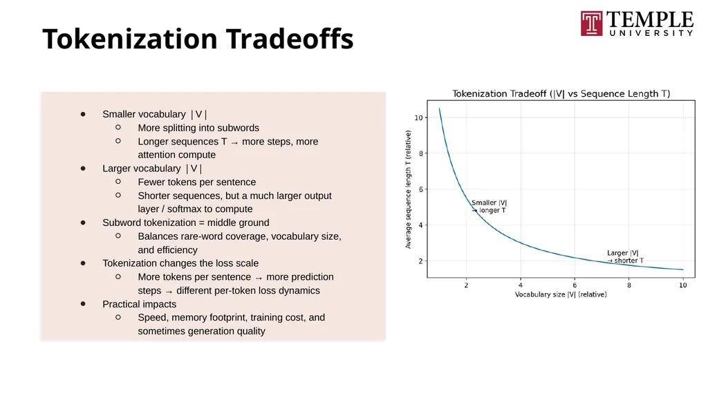
Tokenization Tradeoffs Smaller vocabulary ∣V∣
More splitting into subwords
Longer sequences T → more steps, more attention compute
Larger vocabulary ∣V∣
Fewer tokens per sentence
Shorter sequences, but a much larger output layer / softmax to compute
Subword tokenization = middle ground
Balances rare‑word coverage, vocabulary size, and efficiency
Tokenization changes the loss scale
More tokens per sentence → more prediction steps → different per‑token loss dynamics
Practical impacts
Speed, memory footprint, training cost, and sometimes generation quality<br>
More splitting into subwords
Longer sequences T → more steps, more attention compute
Larger vocabulary ∣V∣
Fewer tokens per sentence
Shorter sequences, but a much larger output layer / softmax to compute
Subword tokenization = middle ground
Balances rare‑word coverage, vocabulary size, and efficiency
Tokenization changes the loss scale
More tokens per sentence → more prediction steps → different per‑token loss dynamics
Practical impacts
Speed, memory footprint, training cost, and sometimes generation quality<br>
11
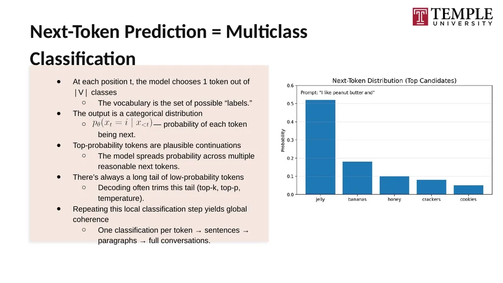
Next-Token Prediction = Multiclass Classification At each position t, the model chooses 1 token out of ∣V∣ classes
The vocabulary is the set of possible “labels.”
The output is a categorical distribution
— probability of each token being next.
Top‑probability tokens are plausible continuations
The model spreads probability across multiple reasonable next tokens.
There’s always a long tail of low‑probability tokens
Decoding often trims this tail (top‑k, top‑p, temperature).
Repeating this local classification step yields global coherence
One classification per token → sentences → paragraphs → full conversations.<br>
The vocabulary is the set of possible “labels.”
The output is a categorical distribution
— probability of each token being next.
Top‑probability tokens are plausible continuations
The model spreads probability across multiple reasonable next tokens.
There’s always a long tail of low‑probability tokens
Decoding often trims this tail (top‑k, top‑p, temperature).
Repeating this local classification step yields global coherence
One classification per token → sentences → paragraphs → full conversations.<br>
12
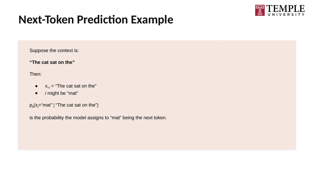
Next-Token Prediction Example Suppose the context is:
“The cat sat on the”
Then:
x<t = “The cat sat on the”
i might be “mat”
pθ(xt=“mat”∣“The cat sat on the”)
is the probability the model assigns to “mat” being the next token.<br>
“The cat sat on the”
Then:
x<t = “The cat sat on the”
i might be “mat”
pθ(xt=“mat”∣“The cat sat on the”)
is the probability the model assigns to “mat” being the next token.<br>
13
Autoregressive Modeling (Core Idea) LLMs generate text left‑to‑right
Standard setup: each position depends on all earlier tokens.
Each new token is predicted from the full context
“Given everything so far, what comes next?”
Generated tokens are fed back into the model
Predict → append → use as new context → repeat.
Decisions are path‑dependent
Early tokens influence all later predictions.
Autoregression enables streaming and long‑form generation
The model can produce text one token at a time, indefinitely.<br>
Standard setup: each position depends on all earlier tokens.
Each new token is predicted from the full context
“Given everything so far, what comes next?”
Generated tokens are fed back into the model
Predict → append → use as new context → repeat.
Decisions are path‑dependent
Early tokens influence all later predictions.
Autoregression enables streaming and long‑form generation
The model can produce text one token at a time, indefinitely.<br>
14
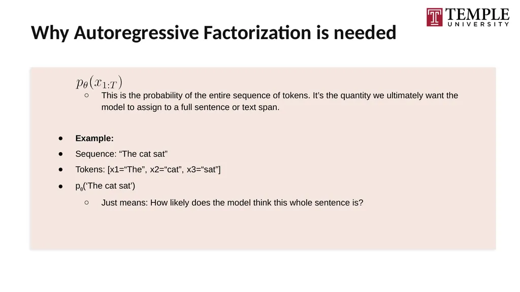
Why Autoregressive Factorization is needed This is the probability of the entire sequence of tokens. It’s the quantity we ultimately want the model to assign to a full sentence or text span.
Example:
Sequence: “The cat sat”
Tokens: [x1=“The”, x2=“cat”, x3=“sat”]
pθ(‘The cat sat’)
Just means: How likely does the model think this whole sentence is?<br>
Example:
Sequence: “The cat sat”
Tokens: [x1=“The”, x2=“cat”, x3=“sat”]
pθ(‘The cat sat’)
Just means: How likely does the model think this whole sentence is?<br>
15
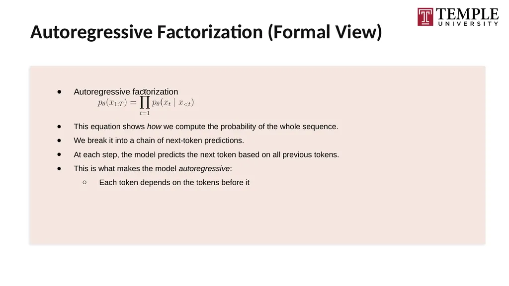
Autoregressive Factorization (Formal View) Autoregressive factorization
This equation shows how we compute the probability of the whole sequence.
We break it into a chain of next‑token predictions.
At each step, the model predicts the next token based on all previous tokens.
This is what makes the model autoregressive:
Each token depends on the tokens before it<br>
This equation shows how we compute the probability of the whole sequence.
We break it into a chain of next‑token predictions.
At each step, the model predicts the next token based on all previous tokens.
This is what makes the model autoregressive:
Each token depends on the tokens before it<br>
16
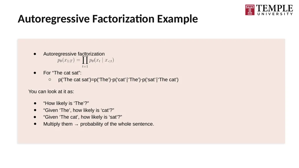
Autoregressive Factorization Example Autoregressive factorization
For “The cat sat”:
p(‘The cat sat’)=p(‘The’)⋅p(‘cat’∣‘The’)⋅p(‘sat’∣‘The cat’)
You can look at it as:
“How likely is ‘The’?”
“Given ‘The’, how likely is ‘cat’?”
“Given ‘The cat’, how likely is ‘sat’?”
Multiply them → probability of the whole sentence.<br>
For “The cat sat”:
p(‘The cat sat’)=p(‘The’)⋅p(‘cat’∣‘The’)⋅p(‘sat’∣‘The cat’)
You can look at it as:
“How likely is ‘The’?”
“Given ‘The’, how likely is ‘cat’?”
“Given ‘The cat’, how likely is ‘sat’?”
Multiply them → probability of the whole sentence.<br>
17
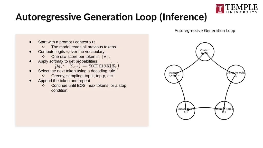
Autoregressive Generation Loop (Inference) Start with a prompt / context x<t
The model reads all previous tokens.
Compute logits over the vocabulary
One raw score per token in ∣V∣.
Apply softmax to get probabilities
Select the next token using a decoding rule
Greedy, sampling, top‑k, top‑p, etc.
Append the token and repeat
Continue until EOS, max tokens, or a stop condition.<br>
The model reads all previous tokens.
Compute logits over the vocabulary
One raw score per token in ∣V∣.
Apply softmax to get probabilities
Select the next token using a decoding rule
Greedy, sampling, top‑k, top‑p, etc.
Append the token and repeat
Continue until EOS, max tokens, or a stop condition.<br>
18
Training vs Inference: Teacher Forcing & Exposure Bias Training uses ground‑truth prefixes (teacher forcing)
The model conditions on real prefixes x<t from the dataset.
Targets are known during training
The next token xt comes directly from real text.
Inference uses model‑generated prefixes
The model conditions on its own predictions
This mismatch can cause error compounding (exposure bias)
Small mistakes early on can snowball into larger deviations.
Long‑horizon generation is more vulnerable
Drift, instability, and off‑distribution behavior become more likely.<br>
The model conditions on real prefixes x<t from the dataset.
Targets are known during training
The next token xt comes directly from real text.
Inference uses model‑generated prefixes
The model conditions on its own predictions
This mismatch can cause error compounding (exposure bias)
Small mistakes early on can snowball into larger deviations.
Long‑horizon generation is more vulnerable
Drift, instability, and off‑distribution behavior become more likely.<br>
19
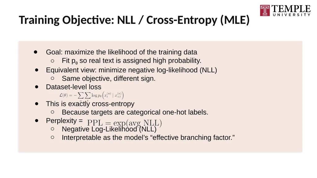
Training Objective: NLL / Cross-Entropy (MLE) Goal: maximize the likelihood of the training data
Fit pθ so real text is assigned high probability.
Equivalent view: minimize negative log‑likelihood (NLL)
Same objective, different sign.
Dataset‑level loss
This is exactly cross‑entropy
Because targets are categorical one‑hot labels.
Perplexity =
Negative Log‑Likelihood (NLL)
Interpretable as the model’s “effective branching factor.”<br>
Fit pθ so real text is assigned high probability.
Equivalent view: minimize negative log‑likelihood (NLL)
Same objective, different sign.
Dataset‑level loss
This is exactly cross‑entropy
Because targets are categorical one‑hot labels.
Perplexity =
Negative Log‑Likelihood (NLL)
Interpretable as the model’s “effective branching factor.”<br>
20
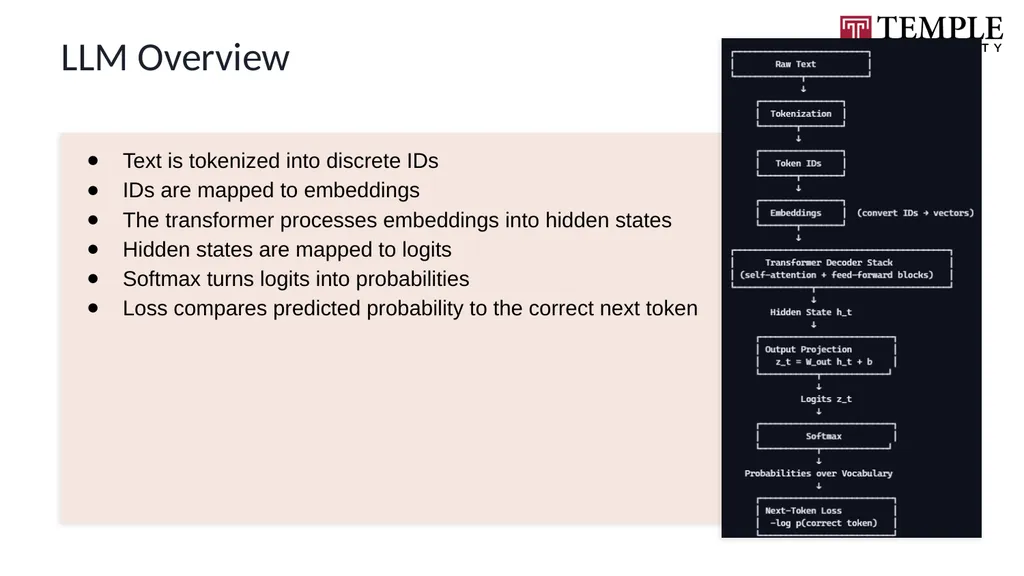
LLM Overview Text is tokenized into discrete IDs
IDs are mapped to embeddings
The transformer processes embeddings into hidden states
Hidden states are mapped to logits
Softmax turns logits into probabilities
Loss compares predicted probability to the correct next token<br>
IDs are mapped to embeddings
The transformer processes embeddings into hidden states
Hidden states are mapped to logits
Softmax turns logits into probabilities
Loss compares predicted probability to the correct next token<br>
21
Intro to Logits What are logits?
Raw, unnormalized scores the model produces before applying softmax.
Where do they come from?
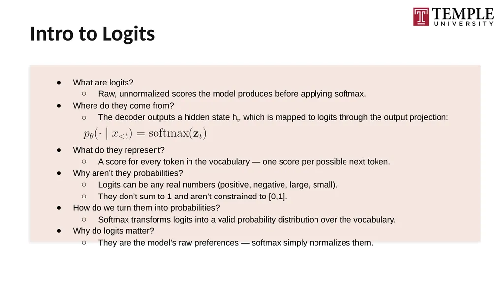
The decoder outputs a hidden state ht, which is mapped to logits through the output projection:
What do they represent?
A score for every token in the vocabulary — one score per possible next token.
Why aren’t they probabilities?
Logits can be any real numbers (positive, negative, large, small).
They don’t sum to 1 and aren’t constrained to [0,1].
How do we turn them into probabilities?
Softmax transforms logits into a valid probability distribution over the vocabulary.
Why do logits matter?
They are the model’s raw preferences — softmax simply normalizes them.<br>
Raw, unnormalized scores the model produces before applying softmax.
Where do they come from?
The decoder outputs a hidden state ht, which is mapped to logits through the output projection:
What do they represent?
A score for every token in the vocabulary — one score per possible next token.
Why aren’t they probabilities?
Logits can be any real numbers (positive, negative, large, small).
They don’t sum to 1 and aren’t constrained to [0,1].
How do we turn them into probabilities?
Softmax transforms logits into a valid probability distribution over the vocabulary.
Why do logits matter?
They are the model’s raw preferences — softmax simply normalizes them.<br>
22
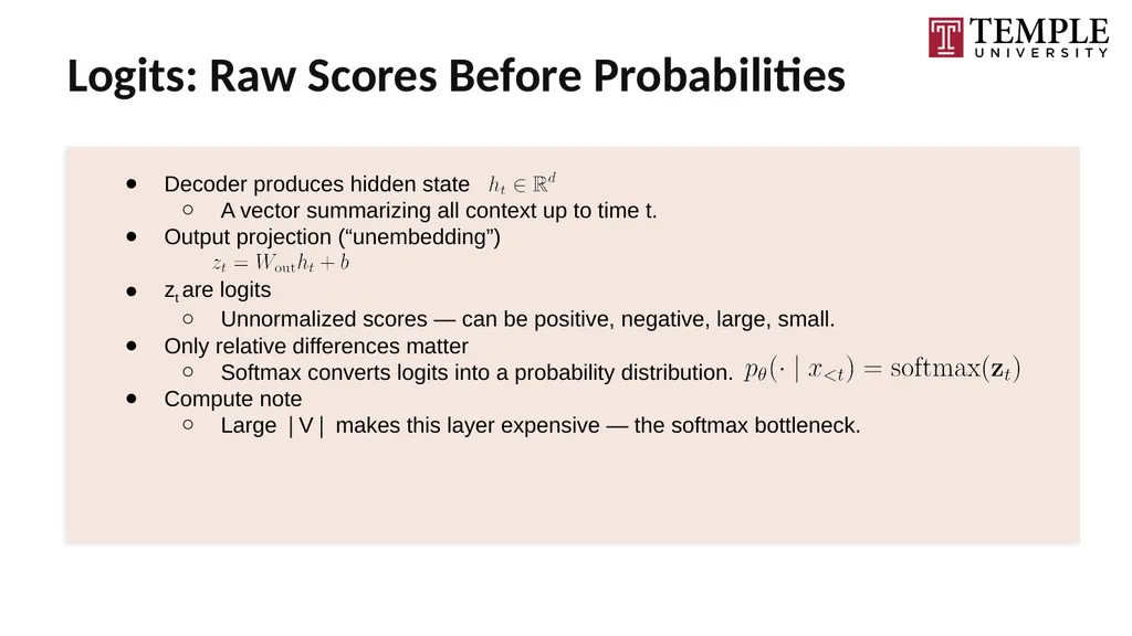
Logits: Raw Scores Before Probabilities Decoder produces hidden state
A vector summarizing all context up to time t.
Output projection (“unembedding”)
zt are logits
Unnormalized scores — can be positive, negative, large, small.
Only relative differences matter
Softmax converts logits into a probability distribution.
Compute note
Large ∣V∣ makes this layer expensive — the softmax bottleneck.<br>
A vector summarizing all context up to time t.
Output projection (“unembedding”)
zt are logits
Unnormalized scores — can be positive, negative, large, small.
Only relative differences matter
Softmax converts logits into a probability distribution.
Compute note
Large ∣V∣ makes this layer expensive — the softmax bottleneck.<br>
23
Intro to Softmax What does softmax do?
Turns logits into a valid probability distribution.
Why do we need it?
Logits can be any real numbers — softmax normalizes them so probabilities are between 0 and 1 and sum to 1.
Intuition
Exponentials amplify differences in logits: higher logits → much higher probabilities.
What we get
A categorical distribution over the vocabulary — one probability per possible next token.
Why it matters
This is the distribution the model samples from to choose the next token.<br>
Turns logits into a valid probability distribution.
Why do we need it?
Logits can be any real numbers — softmax normalizes them so probabilities are between 0 and 1 and sum to 1.
Intuition
Exponentials amplify differences in logits: higher logits → much higher probabilities.
What we get
A categorical distribution over the vocabulary — one probability per possible next token.
Why it matters
This is the distribution the model samples from to choose the next token.<br>
24
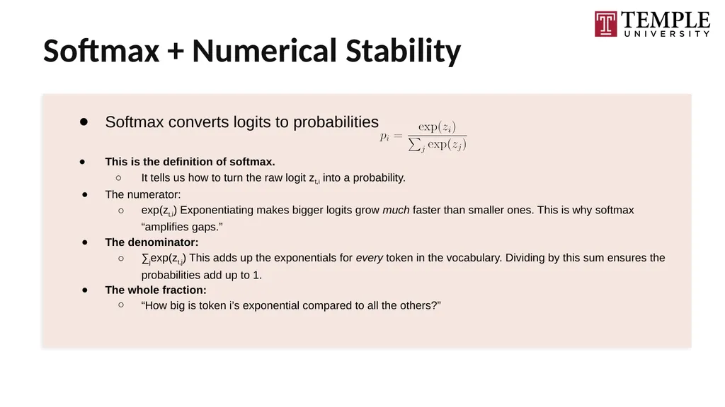
Softmax + Numerical Stability Softmax converts logits to probabilities
This is the definition of softmax.
It tells us how to turn the raw logit zt,i into a probability.
The numerator:
exp(zt,i) Exponentiating makes bigger logits grow much faster than smaller ones. This is why softmax “amplifies gaps.”
The denominator:
∑jexp(zt,j) This adds up the exponentials for every token in the vocabulary. Dividing by this sum ensures the probabilities add up to 1.
The whole fraction:
“How big is token i’s exponential compared to all the others?”<br>
This is the definition of softmax.
It tells us how to turn the raw logit zt,i into a probability.
The numerator:
exp(zt,i) Exponentiating makes bigger logits grow much faster than smaller ones. This is why softmax “amplifies gaps.”
The denominator:
∑jexp(zt,j) This adds up the exponentials for every token in the vocabulary. Dividing by this sum ensures the probabilities add up to 1.
The whole fraction:
“How big is token i’s exponential compared to all the others?”<br>
25
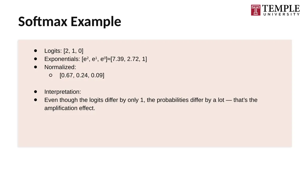
Softmax Example Logits: [2, 1, 0]
Exponentials: [e2, e1, e0]≈[7.39, 2.72, 1]
Normalized:
[0.67, 0.24, 0.09]
Interpretation:
Even though the logits differ by only 1, the probabilities differ by a lot — that’s the amplification effect.<br>
Exponentials: [e2, e1, e0]≈[7.39, 2.72, 1]
Normalized:
[0.67, 0.24, 0.09]
Interpretation:
Even though the logits differ by only 1, the probabilities differ by a lot — that’s the amplification effect.<br>
26
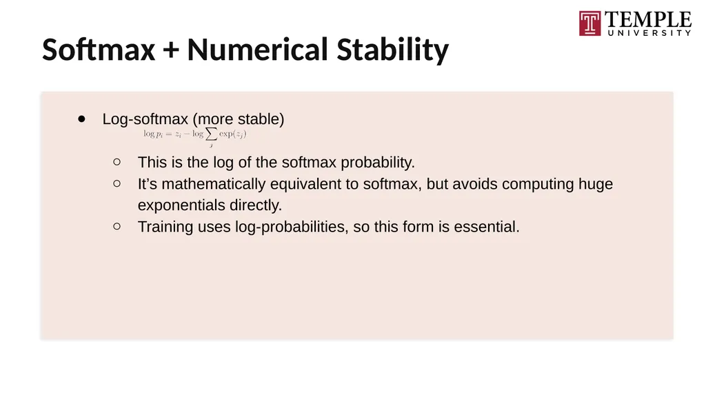
Softmax + Numerical Stability Log‑softmax (more stable)
This is the log of the softmax probability.
It’s mathematically equivalent to softmax, but avoids computing huge exponentials directly.
Training uses log‑probabilities, so this form is essential.<br>
This is the log of the softmax probability.
It’s mathematically equivalent to softmax, but avoids computing huge exponentials directly.
Training uses log‑probabilities, so this form is essential.<br>
27
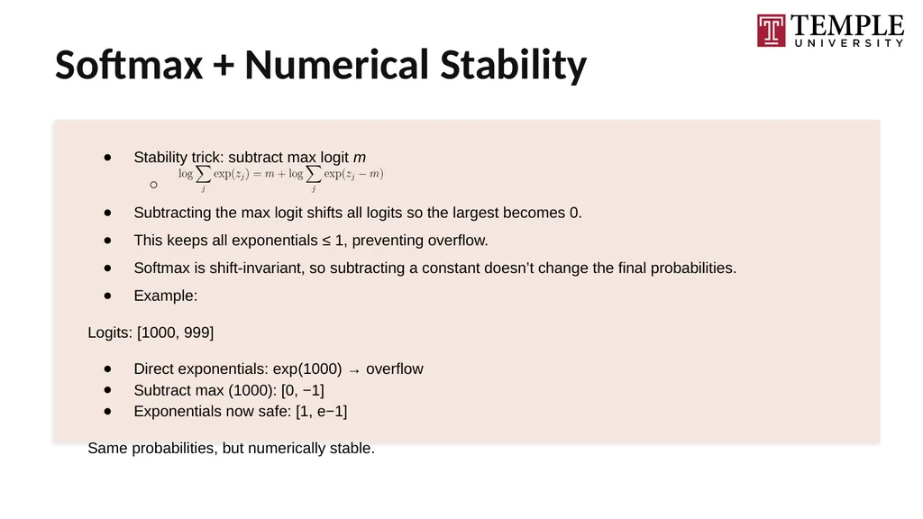
Softmax + Numerical Stability Stability trick: subtract max logit m
Subtracting the max logit shifts all logits so the largest becomes 0.
This keeps all exponentials ≤ 1, preventing overflow.
Softmax is shift‑invariant, so subtracting a constant doesn’t change the final probabilities.
Example:
Logits: [1000, 999]
Direct exponentials: exp(1000) → overflow
Subtract max (1000): [0, −1]
Exponentials now safe: [1, e−1]
Same probabilities, but numerically stable.<br>
Subtracting the max logit shifts all logits so the largest becomes 0.
This keeps all exponentials ≤ 1, preventing overflow.
Softmax is shift‑invariant, so subtracting a constant doesn’t change the final probabilities.
Example:
Logits: [1000, 999]
Direct exponentials: exp(1000) → overflow
Subtract max (1000): [0, −1]
Exponentials now safe: [1, e−1]
Same probabilities, but numerically stable.<br>
28
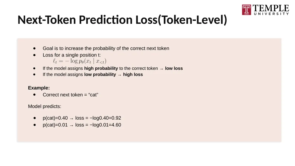
Next-Token Prediction Loss(Token-Level) Goal is to increase the probability of the correct next token
Loss for a single position t:
If the model assigns high probability to the correct token → low loss
If the model assigns low probability → high loss
Example:
Correct next token = “cat”
Model predicts:
p(cat)=0.40 → loss = −log0.40=0.92
p(cat)=0.01 → loss = −log0.01=4.60<br>
Loss for a single position t:
If the model assigns high probability to the correct token → low loss
If the model assigns low probability → high loss
Example:
Correct next token = “cat”
Model predicts:
p(cat)=0.40 → loss = −log0.40=0.92
p(cat)=0.01 → loss = −log0.01=4.60<br>
29
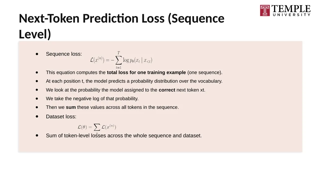
Next-Token Prediction Loss (Sequence Level) Sequence loss:
This equation computes the total loss for one training example (one sequence).
At each position t, the model predicts a probability distribution over the vocabulary.
We look at the probability the model assigned to the correct next token xt.
We take the negative log of that probability.
Then we sum these values across all tokens in the sequence.
Dataset loss:
Sum of token‑level losses across the whole sequence and dataset.<br>
This equation computes the total loss for one training example (one sequence).
At each position t, the model predicts a probability distribution over the vocabulary.
We look at the probability the model assigned to the correct next token xt.
We take the negative log of that probability.
Then we sum these values across all tokens in the sequence.
Dataset loss:
Sum of token‑level losses across the whole sequence and dataset.<br>
30
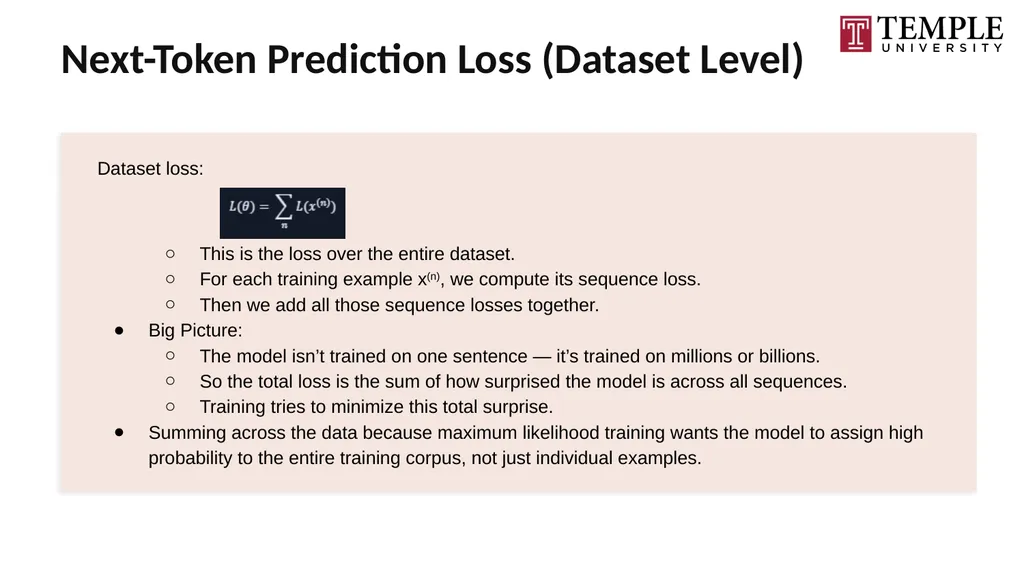
Next-Token Prediction Loss (Dataset Level) Dataset loss:
This is the loss over the entire dataset.
For each training example x(n), we compute its sequence loss.
Then we add all those sequence losses together.
Big Picture:
The model isn’t trained on one sentence — it’s trained on millions or billions.
So the total loss is the sum of how surprised the model is across all sequences.
Training tries to minimize this total surprise.
Summing across the data because maximum likelihood training wants the model to assign high probability to the entire training corpus, not just individual examples.<br>
This is the loss over the entire dataset.
For each training example x(n), we compute its sequence loss.
Then we add all those sequence losses together.
Big Picture:
The model isn’t trained on one sentence — it’s trained on millions or billions.
So the total loss is the sum of how surprised the model is across all sequences.
Training tries to minimize this total surprise.
Summing across the data because maximum likelihood training wants the model to assign high probability to the entire training corpus, not just individual examples.<br>
31
Part 2:
Prompting and
Conditioning How we communicate with LLMs and steer their behavior<br>
Prompting and
Conditioning How we communicate with LLMs and steer their behavior<br>
32
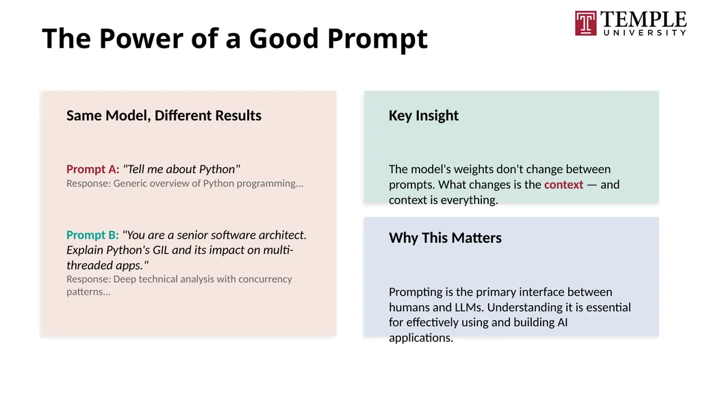
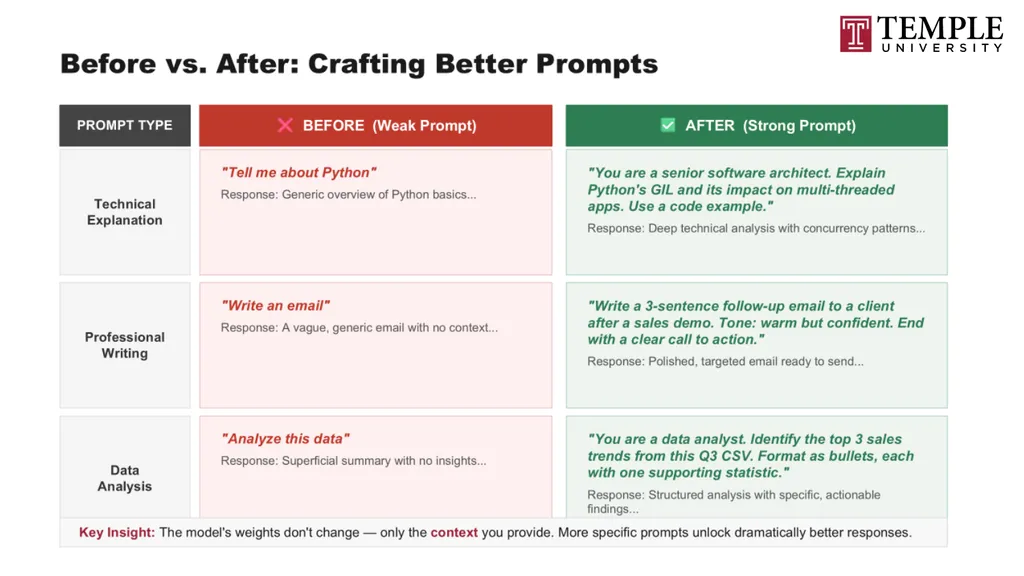
The Power of a Good Prompt Same Model, Different Results
Prompt A: "Tell me about Python"
Response: Generic overview of Python programming...
Prompt B: "You are a senior software architect. Explain Python's GIL and its impact on multi-threaded apps."
Response: Deep technical analysis with concurrency patterns... Key Insight
The model's weights don't change between prompts. What changes is the context — and context is everything. Why This Matters
Prompting is the primary interface between humans and LLMs. Understanding it is essential for effectively using and building AI applications.<br>
Prompt A: "Tell me about Python"
Response: Generic overview of Python programming...
Prompt B: "You are a senior software architect. Explain Python's GIL and its impact on multi-threaded apps."
Response: Deep technical analysis with concurrency patterns... Key Insight
The model's weights don't change between prompts. What changes is the context — and context is everything. Why This Matters
Prompting is the primary interface between humans and LLMs. Understanding it is essential for effectively using and building AI applications.<br>
33
What is In-Context Learning? Definition
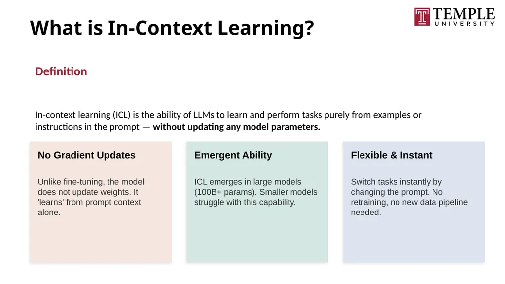
In-context learning (ICL) is the ability of LLMs to learn and perform tasks purely from examples or instructions in the prompt — without updating any model parameters. No Gradient Updates Unlike fine-tuning, the model does not update weights. It 'learns' from prompt context alone. Emergent Ability ICL emerges in large models (100B+ params). Smaller models struggle with this capability. Flexible & Instant Switch tasks instantly by changing the prompt. No retraining, no new data pipeline needed.<br>
In-context learning (ICL) is the ability of LLMs to learn and perform tasks purely from examples or instructions in the prompt — without updating any model parameters. No Gradient Updates Unlike fine-tuning, the model does not update weights. It 'learns' from prompt context alone. Emergent Ability ICL emerges in large models (100B+ params). Smaller models struggle with this capability. Flexible & Instant Switch tasks instantly by changing the prompt. No retraining, no new data pipeline needed.<br>
34
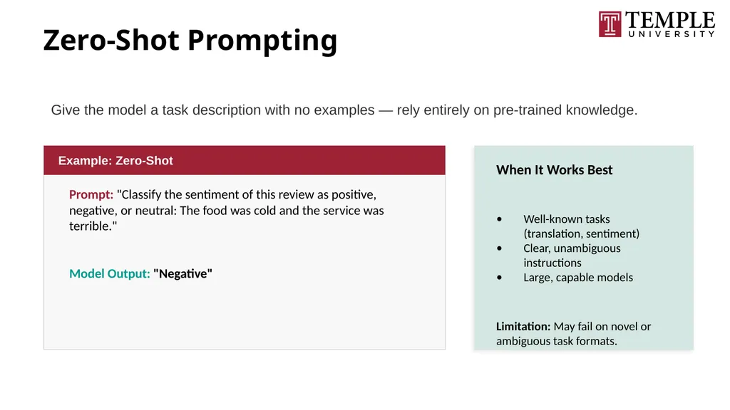
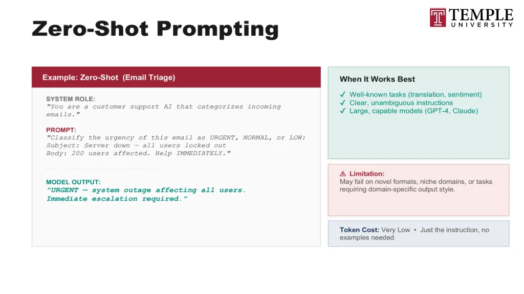
Zero-Shot Prompting Give the model a task description with no examples — rely entirely on pre-trained knowledge. Example: Zero-Shot Prompt: "Classify the sentiment of this review as positive, negative, or neutral: The food was cold and the service was terrible."
Model Output: "Negative" When It Works Best
Well-known tasks (translation, sentiment)
Clear, unambiguous instructions
Large, capable models
Limitation: May fail on novel or ambiguous task formats.<br>
Model Output: "Negative" When It Works Best
Well-known tasks (translation, sentiment)
Clear, unambiguous instructions
Large, capable models
Limitation: May fail on novel or ambiguous task formats.<br>
35
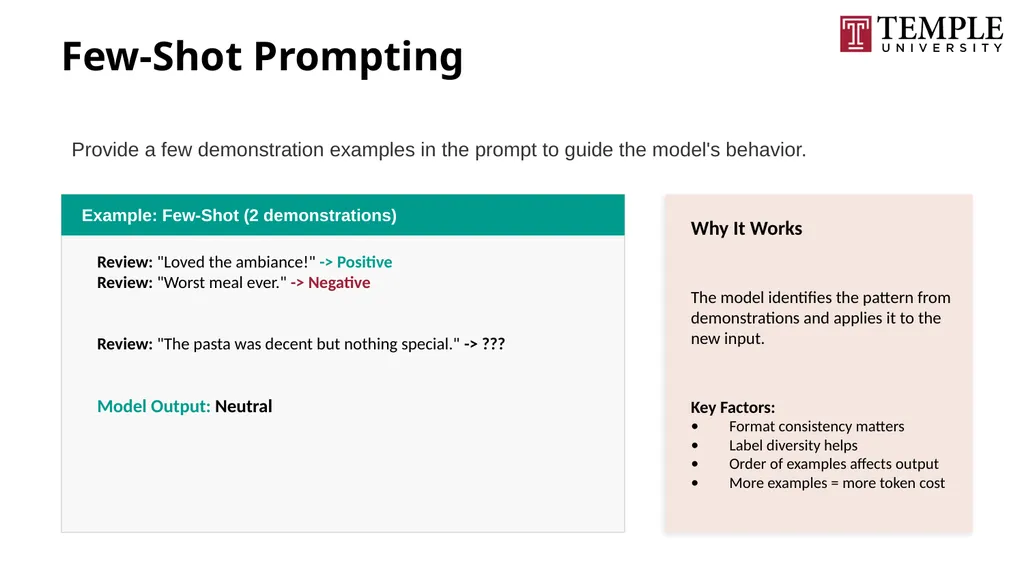
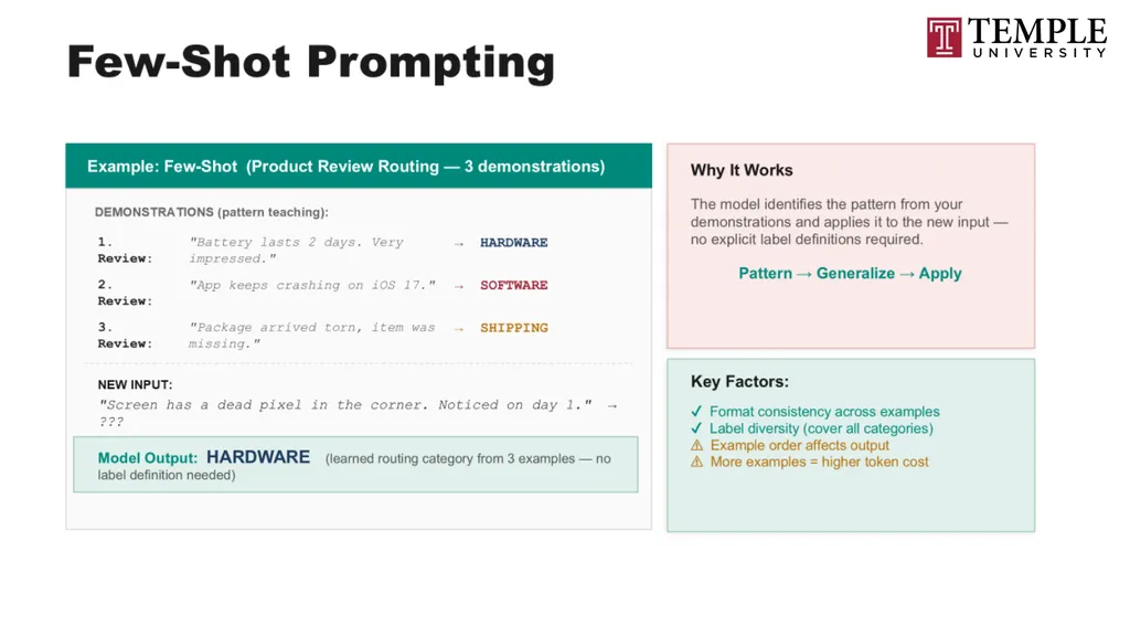
Few-Shot Prompting Provide a few demonstration examples in the prompt to guide the model's behavior. Example: Few-Shot (2 demonstrations) Review: "Loved the ambiance!" -> Positive
Review: "Worst meal ever." -> Negative
Review: "The pasta was decent but nothing special." -> ???
Model Output: Neutral Why It Works
The model identifies the pattern from demonstrations and applies it to the new input.
Key Factors:
Format consistency matters
Label diversity helps
Order of examples affects output
More examples = more token cost<br>
Review: "Worst meal ever." -> Negative
Review: "The pasta was decent but nothing special." -> ???
Model Output: Neutral Why It Works
The model identifies the pattern from demonstrations and applies it to the new input.
Key Factors:
Format consistency matters
Label diversity helps
Order of examples affects output
More examples = more token cost<br>
36
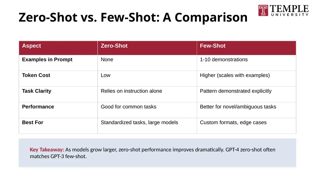
Zero-Shot vs. Few-Shot: A Comparison Key Takeaway: As models grow larger, zero-shot performance improves dramatically. GPT-4 zero-shot often matches GPT-3 few-shot.<br>
37
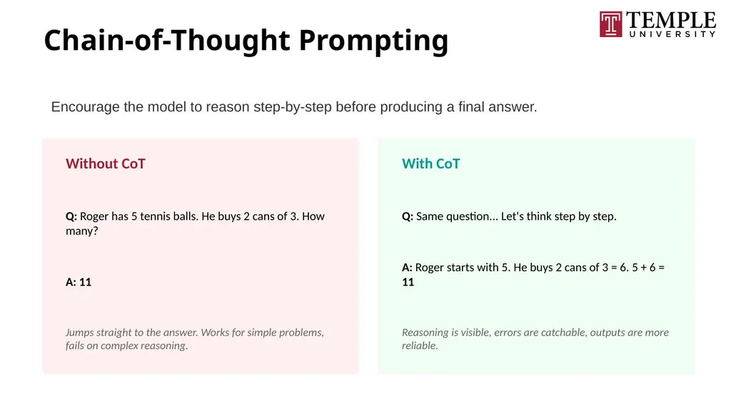
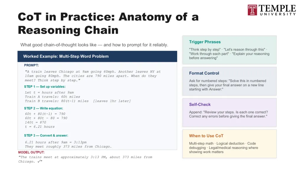
Chain-of-Thought Prompting Encourage the model to reason step-by-step before producing a final answer. Without CoT
Q: Roger has 5 tennis balls. He buys 2 cans of 3. How many?
A: 11
Jumps straight to the answer. Works for simple problems, fails on complex reasoning. With CoT
Q: Same question... Let's think step by step.
A: Roger starts with 5. He buys 2 cans of 3 = 6. 5 + 6 = 11
Reasoning is visible, errors are catchable, outputs are more reliable.<br>
Q: Roger has 5 tennis balls. He buys 2 cans of 3. How many?
A: 11
Jumps straight to the answer. Works for simple problems, fails on complex reasoning. With CoT
Q: Same question... Let's think step by step.
A: Roger starts with 5. He buys 2 cans of 3 = 6. 5 + 6 = 11
Reasoning is visible, errors are catchable, outputs are more reliable.<br>
38
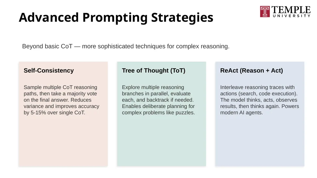
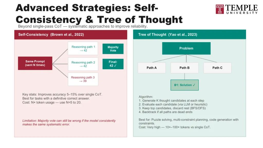
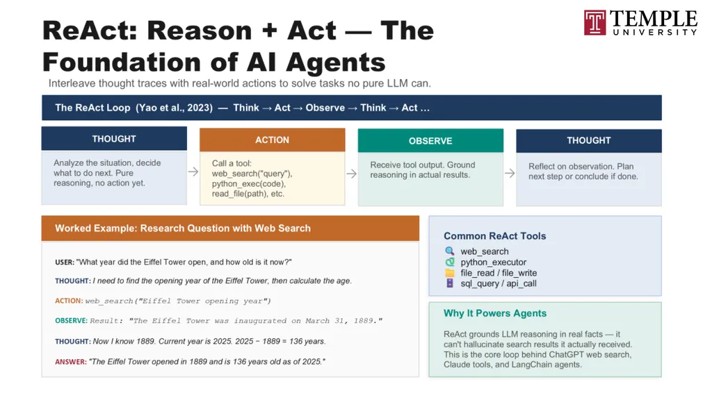
Advanced Prompting Strategies Beyond basic CoT — more sophisticated techniques for complex reasoning. Self-Consistency Sample multiple CoT reasoning paths, then take a majority vote on the final answer. Reduces variance and improves accuracy by 5-15% over single CoT. Tree of Thought (ToT) Explore multiple reasoning branches in parallel, evaluate each, and backtrack if needed. Enables deliberate planning for complex problems like puzzles. ReAct (Reason + Act) Interleave reasoning traces with actions (search, code execution). The model thinks, acts, observes results, then thinks again. Powers modern AI agents.<br>
39
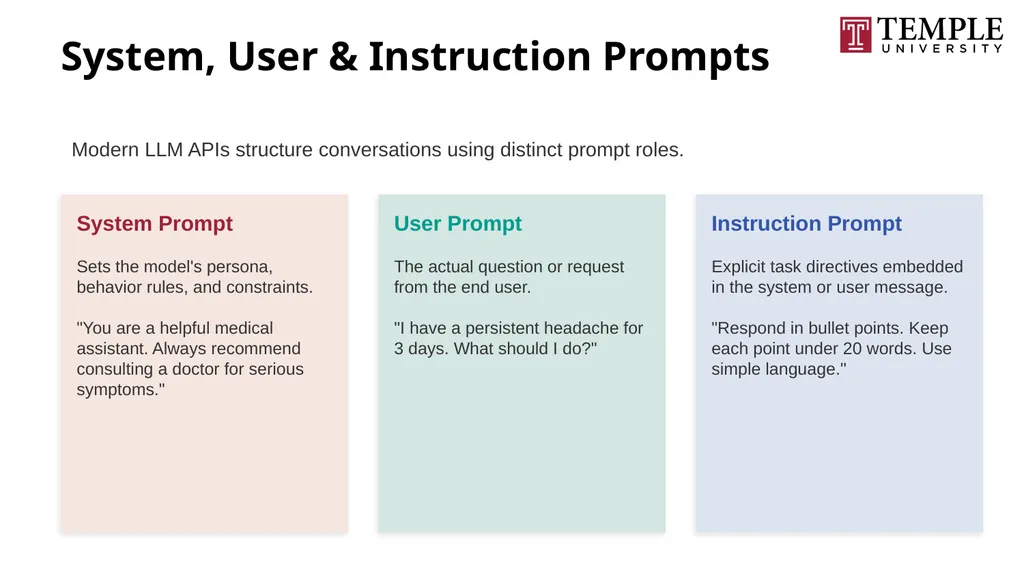
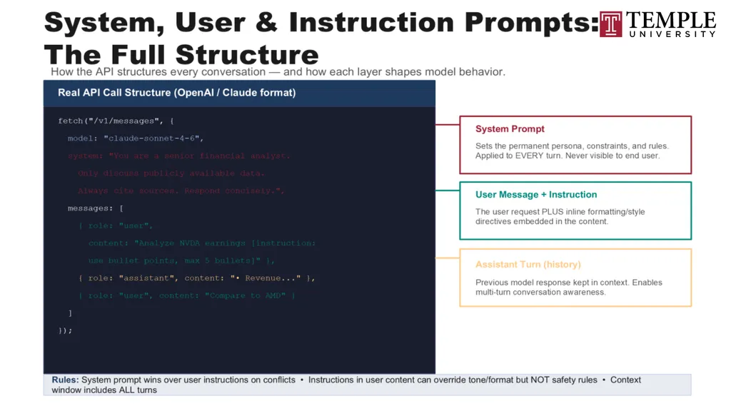
System, User & Instruction Prompts Modern LLM APIs structure conversations using distinct prompt roles. System Prompt Sets the model's persona, behavior rules, and constraints.
"You are a helpful medical assistant. Always recommend consulting a doctor for serious symptoms." User Prompt The actual question or request from the end user.
"I have a persistent headache for 3 days. What should I do?" Instruction Prompt Explicit task directives embedded in the system or user message.
"Respond in bullet points. Keep each point under 20 words. Use simple language."<br>
"You are a helpful medical assistant. Always recommend consulting a doctor for serious symptoms." User Prompt The actual question or request from the end user.
"I have a persistent headache for 3 days. What should I do?" Instruction Prompt Explicit task directives embedded in the system or user message.
"Respond in bullet points. Keep each point under 20 words. Use simple language."<br>
40
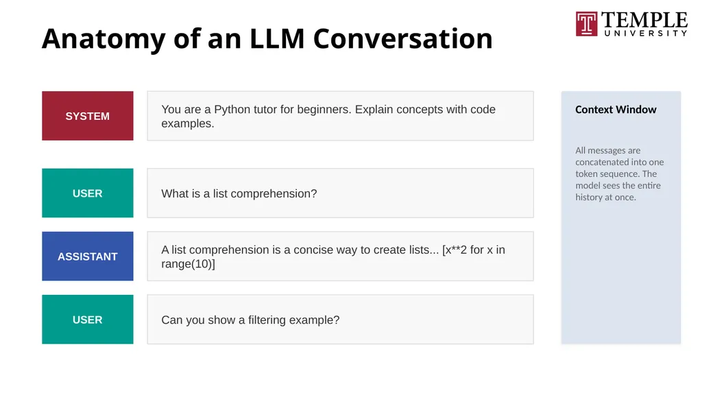
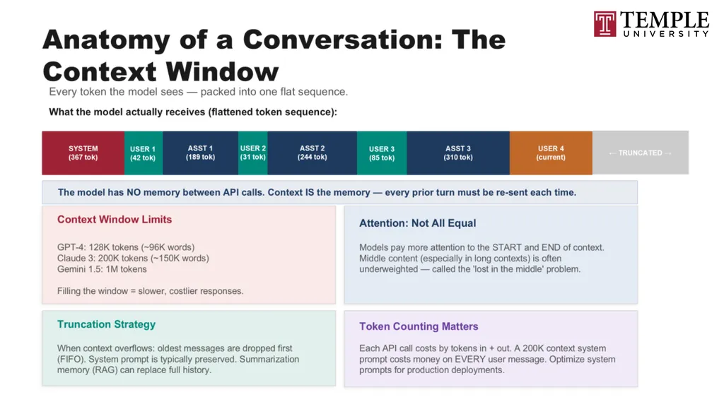
Anatomy of an LLM Conversation SYSTEM You are a Python tutor for beginners. Explain concepts with code examples. USER What is a list comprehension? ASSISTANT A list comprehension is a concise way to create lists... [x**2 for x in range(10)] USER Can you show a filtering example? Context Window
All messages are concatenated into one token sequence. The model sees the entire history at once.<br>
All messages are concatenated into one token sequence. The model sees the entire history at once.<br>
41
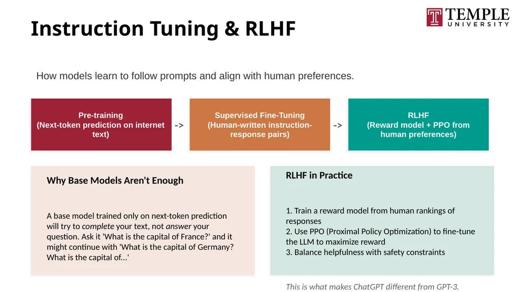
Instruction Tuning & RLHF How models learn to follow prompts and align with human preferences. Pre-training
(Next-token prediction on internet text) -> Supervised Fine-Tuning
(Human-written instruction-response pairs) -> RLHF
(Reward model + PPO from human preferences) Why Base Models Aren't Enough
A base model trained only on next-token prediction will try to complete your text, not answer your question. Ask it 'What is the capital of France?' and it might continue with 'What is the capital of Germany? What is the capital of...' RLHF in Practice
1. Train a reward model from human rankings of responses
2. Use PPO (Proximal Policy Optimization) to fine-tune the LLM to maximize reward
3. Balance helpfulness with safety constraints
This is what makes ChatGPT different from GPT-3.<br>
(Next-token prediction on internet text) -> Supervised Fine-Tuning
(Human-written instruction-response pairs) -> RLHF
(Reward model + PPO from human preferences) Why Base Models Aren't Enough
A base model trained only on next-token prediction will try to complete your text, not answer your question. Ask it 'What is the capital of France?' and it might continue with 'What is the capital of Germany? What is the capital of...' RLHF in Practice
1. Train a reward model from human rankings of responses
2. Use PPO (Proximal Policy Optimization) to fine-tune the LLM to maximize reward
3. Balance helpfulness with safety constraints
This is what makes ChatGPT different from GPT-3.<br>
42
Part 3:
Architectural
Components Inside the Transformer Decoder — embeddings, attention, and the path from tokens to predictions<br>
Architectural
Components Inside the Transformer Decoder — embeddings, attention, and the path from tokens to predictions<br>
43
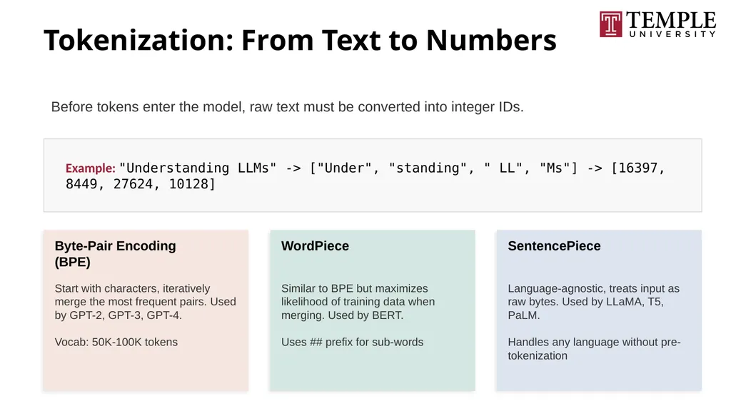
Tokenization: From Text to Numbers Before tokens enter the model, raw text must be converted into integer IDs. Example: "Understanding LLMs" -> ["Under", "standing", " LL", "Ms"] -> [16397, 8449, 27624, 10128] Byte-Pair Encoding
(BPE) Start with characters, iteratively merge the most frequent pairs. Used by GPT-2, GPT-3, GPT-4.
Vocab: 50K-100K tokens WordPiece Similar to BPE but maximizes likelihood of training data when merging. Used by BERT.
Uses ## prefix for sub-words SentencePiece Language-agnostic, treats input as raw bytes. Used by LLaMA, T5, PaLM.
Handles any language without pre-tokenization<br>
(BPE) Start with characters, iteratively merge the most frequent pairs. Used by GPT-2, GPT-3, GPT-4.
Vocab: 50K-100K tokens WordPiece Similar to BPE but maximizes likelihood of training data when merging. Used by BERT.
Uses ## prefix for sub-words SentencePiece Language-agnostic, treats input as raw bytes. Used by LLaMA, T5, PaLM.
Handles any language without pre-tokenization<br>
44
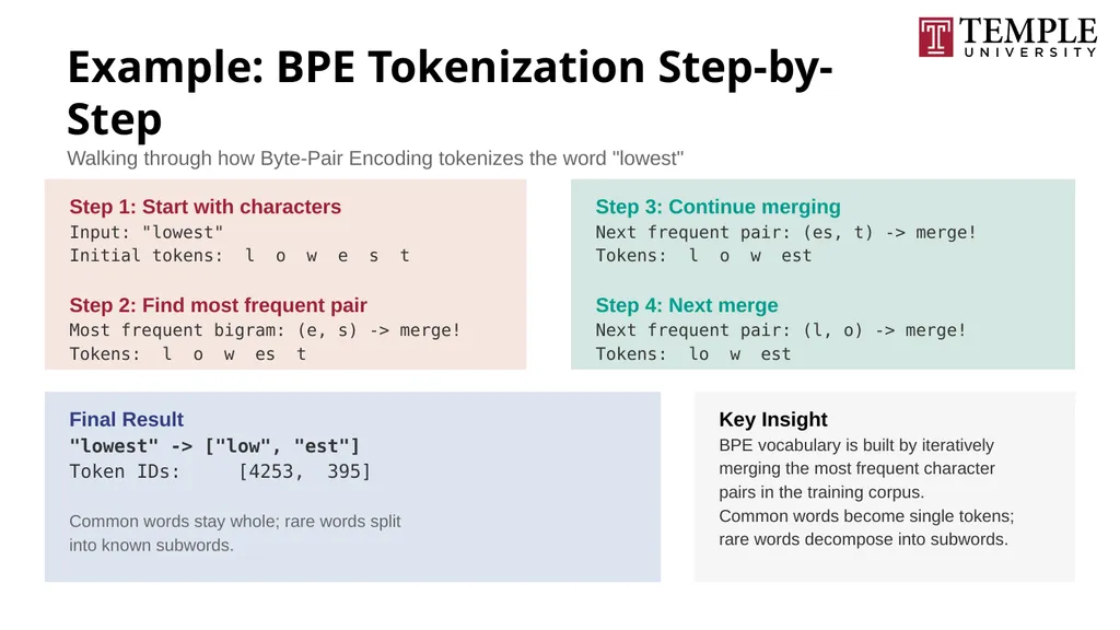
Example: BPE Tokenization Step-by-Step Walking through how Byte-Pair Encoding tokenizes the word "lowest" Step 1: Start with characters
Input: "lowest"
Initial tokens: l o w e s t
Step 2: Find most frequent pair
Most frequent bigram: (e, s) -> merge!
Tokens: l o w es t Step 3: Continue merging
Next frequent pair: (es, t) -> merge!
Tokens: l o w est
Step 4: Next merge
Next frequent pair: (l, o) -> merge!
Tokens: lo w est Final Result
"lowest" -> ["low", "est"]
Token IDs: [4253, 395]
Common words stay whole; rare words split
into known subwords. Key Insight
BPE vocabulary is built by iteratively
merging the most frequent character
pairs in the training corpus.
Common words become single tokens;
rare words decompose into subwords.<br>
Input: "lowest"
Initial tokens: l o w e s t
Step 2: Find most frequent pair
Most frequent bigram: (e, s) -> merge!
Tokens: l o w es t Step 3: Continue merging
Next frequent pair: (es, t) -> merge!
Tokens: l o w est
Step 4: Next merge
Next frequent pair: (l, o) -> merge!
Tokens: lo w est Final Result
"lowest" -> ["low", "est"]
Token IDs: [4253, 395]
Common words stay whole; rare words split
into known subwords. Key Insight
BPE vocabulary is built by iteratively
merging the most frequent character
pairs in the training corpus.
Common words become single tokens;
rare words decompose into subwords.<br>
45
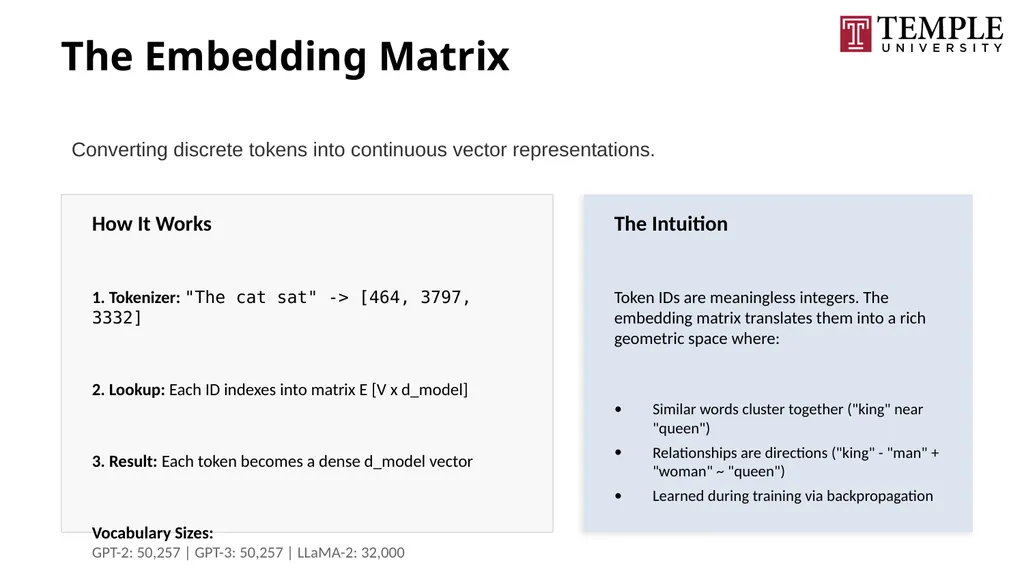
The Embedding Matrix Converting discrete tokens into continuous vector representations. How It Works
1. Tokenizer: "The cat sat" -> [464, 3797, 3332]
2. Lookup: Each ID indexes into matrix E [V x d_model]
3. Result: Each token becomes a dense d_model vector
Vocabulary Sizes:
GPT-2: 50,257 | GPT-3: 50,257 | LLaMA-2: 32,000 The Intuition
Token IDs are meaningless integers. The embedding matrix translates them into a rich geometric space where:
Similar words cluster together ("king" near "queen")
Relationships are directions ("king" - "man" + "woman" ~ "queen")
Learned during training via backpropagation<br>
1. Tokenizer: "The cat sat" -> [464, 3797, 3332]
2. Lookup: Each ID indexes into matrix E [V x d_model]
3. Result: Each token becomes a dense d_model vector
Vocabulary Sizes:
GPT-2: 50,257 | GPT-3: 50,257 | LLaMA-2: 32,000 The Intuition
Token IDs are meaningless integers. The embedding matrix translates them into a rich geometric space where:
Similar words cluster together ("king" near "queen")
Relationships are directions ("king" - "man" + "woman" ~ "queen")
Learned during training via backpropagation<br>
46
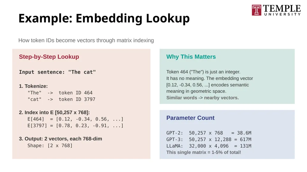
Example: Embedding Lookup How token IDs become vectors through matrix indexing Step-by-Step Lookup
Input sentence: "The cat"
1. Tokenize:
"The" -> token ID 464
"cat" -> token ID 3797
2. Index into E [50,257 x 768]:
E[464] = [0.12, -0.34, 0.56, ...]
E[3797] = [0.78, 0.23, -0.91, ...]
3. Output: 2 vectors, each 768-dim
Shape: [2 x 768] Why This Matters
Token 464 ("The") is just an integer.
It has no meaning. The embedding vector
[0.12, -0.34, 0.56, ...] encodes semantic
meaning in geometric space.
Similar words -> nearby vectors. Parameter Count
GPT-2: 50,257 x 768 = 38.6M
GPT-3: 50,257 x 12,288 = 617M
LLaMA: 32,000 x 4,096 = 131M
This single matrix = 1-5% of total!<br>
Input sentence: "The cat"
1. Tokenize:
"The" -> token ID 464
"cat" -> token ID 3797
2. Index into E [50,257 x 768]:
E[464] = [0.12, -0.34, 0.56, ...]
E[3797] = [0.78, 0.23, -0.91, ...]
3. Output: 2 vectors, each 768-dim
Shape: [2 x 768] Why This Matters
Token 464 ("The") is just an integer.
It has no meaning. The embedding vector
[0.12, -0.34, 0.56, ...] encodes semantic
meaning in geometric space.
Similar words -> nearby vectors. Parameter Count
GPT-2: 50,257 x 768 = 38.6M
GPT-3: 50,257 x 12,288 = 617M
LLaMA: 32,000 x 4,096 = 131M
This single matrix = 1-5% of total!<br>
47
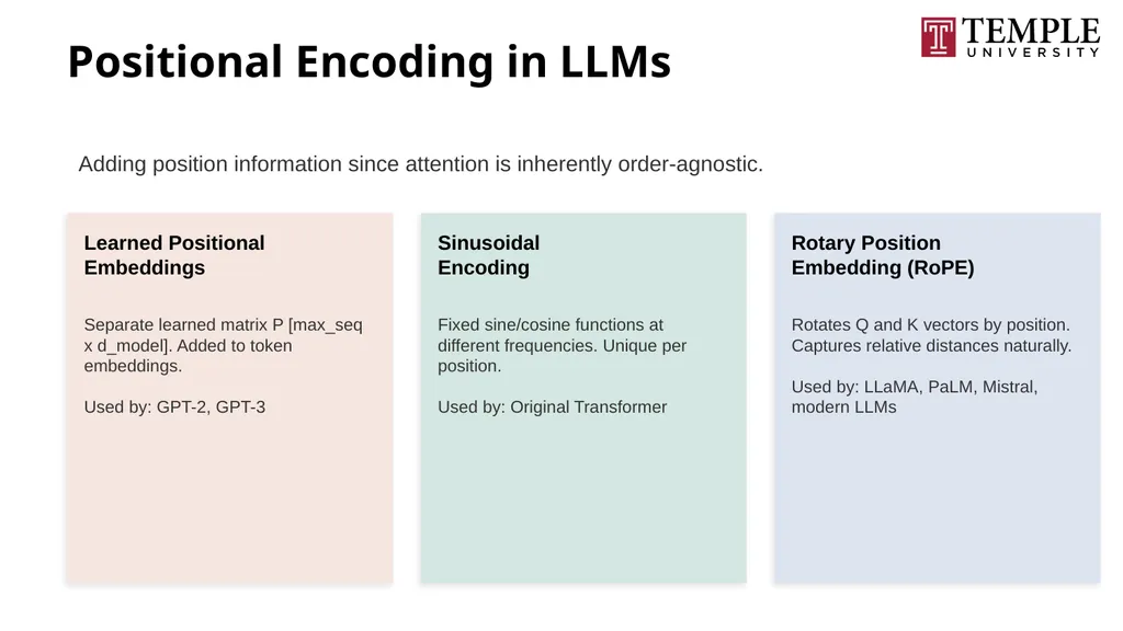
Positional Encoding in LLMs Adding position information since attention is inherently order-agnostic. Learned Positional
Embeddings Separate learned matrix P [max_seq x d_model]. Added to token embeddings.
Used by: GPT-2, GPT-3 Sinusoidal
Encoding Fixed sine/cosine functions at different frequencies. Unique per position.
Used by: Original Transformer Rotary Position
Embedding (RoPE) Rotates Q and K vectors by position. Captures relative distances naturally.
Used by: LLaMA, PaLM, Mistral, modern LLMs<br>
Embeddings Separate learned matrix P [max_seq x d_model]. Added to token embeddings.
Used by: GPT-2, GPT-3 Sinusoidal
Encoding Fixed sine/cosine functions at different frequencies. Unique per position.
Used by: Original Transformer Rotary Position
Embedding (RoPE) Rotates Q and K vectors by position. Captures relative distances naturally.
Used by: LLaMA, PaLM, Mistral, modern LLMs<br>
48
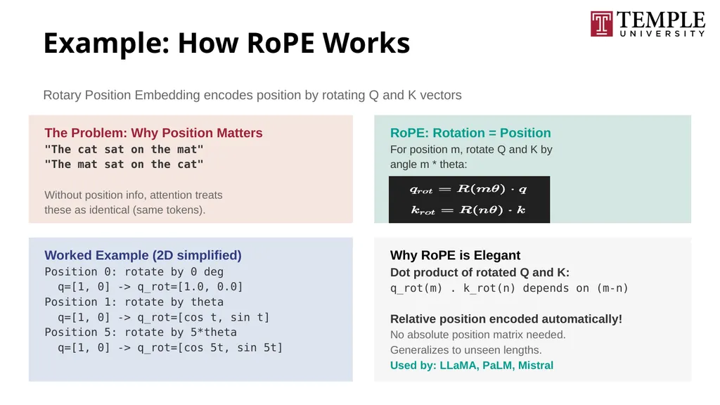
Example: How RoPE Works Rotary Position Embedding encodes position by rotating Q and K vectors The Problem: Why Position Matters
"The cat sat on the mat"
"The mat sat on the cat"
Without position info, attention treats
these as identical (same tokens). RoPE: Rotation = Position
For position m, rotate Q and K by
angle m * theta:
q_rot = R(m * theta) * q
k_rot = R(n * theta) * k Worked Example (2D simplified)
Position 0: rotate by 0 deg
q=[1, 0] -> q_rot=[1.0, 0.0]
Position 1: rotate by theta
q=[1, 0] -> q_rot=[cos t, sin t]
Position 5: rotate by 5*theta
q=[1, 0] -> q_rot=[cos 5t, sin 5t] Why RoPE is Elegant
Dot product of rotated Q and K:
q_rot(m) . k_rot(n) depends on (m-n)
Relative position encoded automatically!
No absolute position matrix needed.
Generalizes to unseen lengths.
Used by: LLaMA, PaLM, Mistral<br>
"The cat sat on the mat"
"The mat sat on the cat"
Without position info, attention treats
these as identical (same tokens). RoPE: Rotation = Position
For position m, rotate Q and K by
angle m * theta:
q_rot = R(m * theta) * q
k_rot = R(n * theta) * k Worked Example (2D simplified)
Position 0: rotate by 0 deg
q=[1, 0] -> q_rot=[1.0, 0.0]
Position 1: rotate by theta
q=[1, 0] -> q_rot=[cos t, sin t]
Position 5: rotate by 5*theta
q=[1, 0] -> q_rot=[cos 5t, sin 5t] Why RoPE is Elegant
Dot product of rotated Q and K:
q_rot(m) . k_rot(n) depends on (m-n)
Relative position encoded automatically!
No absolute position matrix needed.
Generalizes to unseen lengths.
Used by: LLaMA, PaLM, Mistral<br>
49
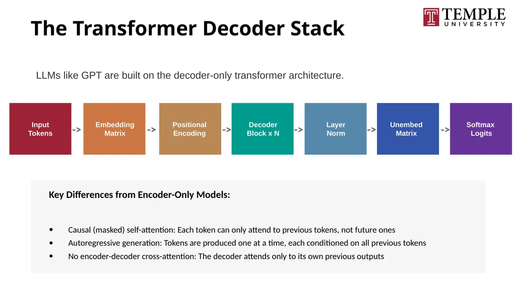
The Transformer Decoder Stack LLMs like GPT are built on the decoder-only transformer architecture. Input
Tokens -> Embedding
Matrix -> Positional
Encoding -> Decoder
Block x N -> Layer
Norm -> Unembed
Matrix Softmax
Logits Key Differences from Encoder-Only Models:
Causal (masked) self-attention: Each token can only attend to previous tokens, not future ones
Autoregressive generation: Tokens are produced one at a time, each conditioned on all previous tokens
No encoder-decoder cross-attention: The decoder attends only to its own previous outputs -><br>
Tokens -> Embedding
Matrix -> Positional
Encoding -> Decoder
Block x N -> Layer
Norm -> Unembed
Matrix Softmax
Logits Key Differences from Encoder-Only Models:
Causal (masked) self-attention: Each token can only attend to previous tokens, not future ones
Autoregressive generation: Tokens are produced one at a time, each conditioned on all previous tokens
No encoder-decoder cross-attention: The decoder attends only to its own previous outputs -><br>
50
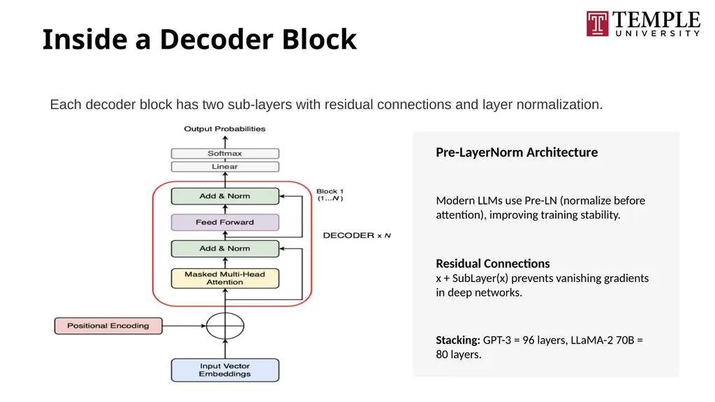
Inside a Decoder Block Each decoder block has two sub-layers with residual connections and layer normalization. Input (from previous layer) Layer Norm Masked Multi-Head Self-Attention Residual Connection (Add) Layer Norm Feed-Forward Network (MLP) Pre-LayerNorm Architecture
Modern LLMs use Pre-LN (normalize before attention), improving training stability.
Residual Connections
x + SubLayer(x) prevents vanishing gradients in deep networks.
Stacking: GPT-3 = 96 layers, LLaMA-2 70B = 80 layers.<br>
Modern LLMs use Pre-LN (normalize before attention), improving training stability.
Residual Connections
x + SubLayer(x) prevents vanishing gradients in deep networks.
Stacking: GPT-3 = 96 layers, LLaMA-2 70B = 80 layers.<br>
51
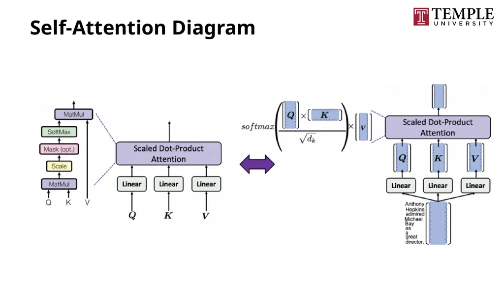
Self-Attention Diagram<br>
52
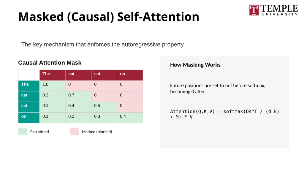
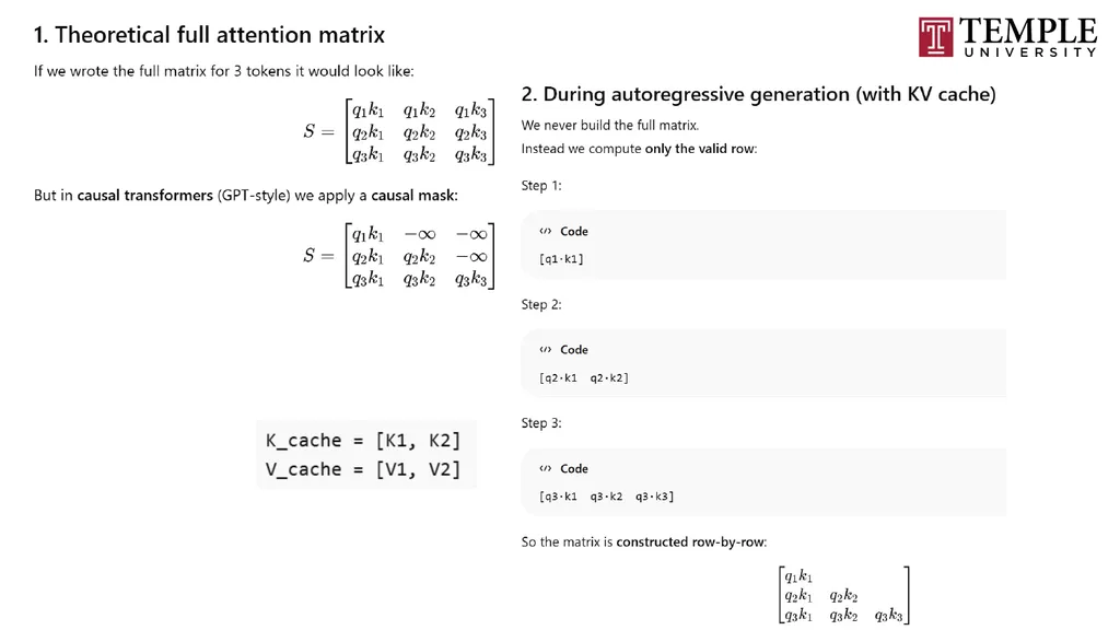
Masked (Causal) Self-Attention The key mechanism that enforces the autoregressive property. Causal Attention Mask Can attend Masked (blocked) How Masking Works
Future positions are set to -inf before softmax, becoming 0 after.
Attention(Q,K,V) = softmax(QK^T / (d_k) + M) * V<br>
Future positions are set to -inf before softmax, becoming 0 after.
Attention(Q,K,V) = softmax(QK^T / (d_k) + M) * V<br>
53
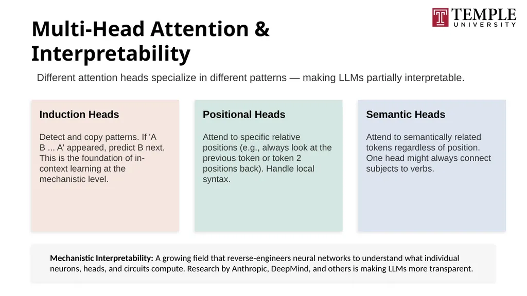
Multi-Head Attention & Interpretability Different attention heads specialize in different patterns — making LLMs partially interpretable. Induction Heads Detect and copy patterns. If 'A B ... A' appeared, predict B next. This is the foundation of in-context learning at the mechanistic level. Positional Heads Attend to specific relative positions (e.g., always look at the previous token or token 2 positions back). Handle local syntax. Semantic Heads Attend to semantically related tokens regardless of position. One head might always connect subjects to verbs. Mechanistic Interpretability: A growing field that reverse-engineers neural networks to understand what individual neurons, heads, and circuits compute. Research by Anthropic, DeepMind, and others is making LLMs more transparent.<br>
54
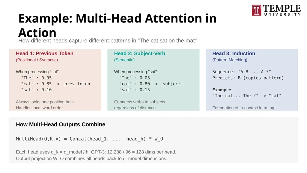
Example: Multi-Head Attention in Action How different heads capture different patterns in "The cat sat on the mat" Head 1: Previous Token
(Positional / Syntactic)
When processing "sat":
"The" : 0.05
"cat" : 0.85 <- prev token
"sat" : 0.10
Always looks one position back.
Handles local word order. Head 2: Subject-Verb
(Semantic)
When processing "sat":
"The" : 0.05
"cat" : 0.80 <- subject!
"sat" : 0.15
Connects verbs to subjects
regardless of distance. Head 3: Induction
(Pattern Matching)
Sequence: "A B ... A ?"
Predicts: B (copies pattern)
Example:
"The cat... The ?" -> "cat"
Foundation of in-context learning! How Multi-Head Outputs Combine
MultiHead(Q,K,V) = Concat(head_1, ..., head_h) * W_O
Each head uses d_k = d_model / h. GPT-3: 12,288 / 96 = 128 dims per head.
Output projection W_O combines all heads back to d_model dimensions.<br>
(Positional / Syntactic)
When processing "sat":
"The" : 0.05
"cat" : 0.85 <- prev token
"sat" : 0.10
Always looks one position back.
Handles local word order. Head 2: Subject-Verb
(Semantic)
When processing "sat":
"The" : 0.05
"cat" : 0.80 <- subject!
"sat" : 0.15
Connects verbs to subjects
regardless of distance. Head 3: Induction
(Pattern Matching)
Sequence: "A B ... A ?"
Predicts: B (copies pattern)
Example:
"The cat... The ?" -> "cat"
Foundation of in-context learning! How Multi-Head Outputs Combine
MultiHead(Q,K,V) = Concat(head_1, ..., head_h) * W_O
Each head uses d_k = d_model / h. GPT-3: 12,288 / 96 = 128 dims per head.
Output projection W_O combines all heads back to d_model dimensions.<br>
55
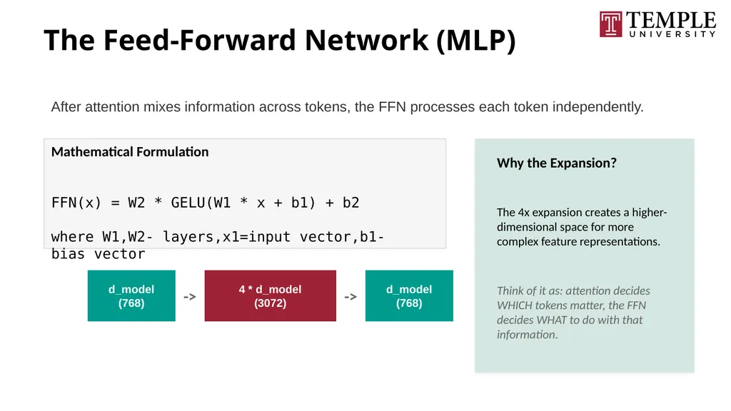
The Feed-Forward Network (MLP) After attention mixes information across tokens, the FFN processes each token independently. Mathematical Formulation
FFN(x) = W2 * GELU(W1 * x + b1) + b2
where W1,W2- layers,x1=input vector,b1- bias vector d_model
(768) -> 4 * d_model
(3072) -> d_model
(768) Why the Expansion?
The 4x expansion creates a higher-dimensional space for more complex feature representations.
Think of it as: attention decides WHICH tokens matter, the FFN decides WHAT to do with that information.<br>
FFN(x) = W2 * GELU(W1 * x + b1) + b2
where W1,W2- layers,x1=input vector,b1- bias vector d_model
(768) -> 4 * d_model
(3072) -> d_model
(768) Why the Expansion?
The 4x expansion creates a higher-dimensional space for more complex feature representations.
Think of it as: attention decides WHICH tokens matter, the FFN decides WHAT to do with that information.<br>
56
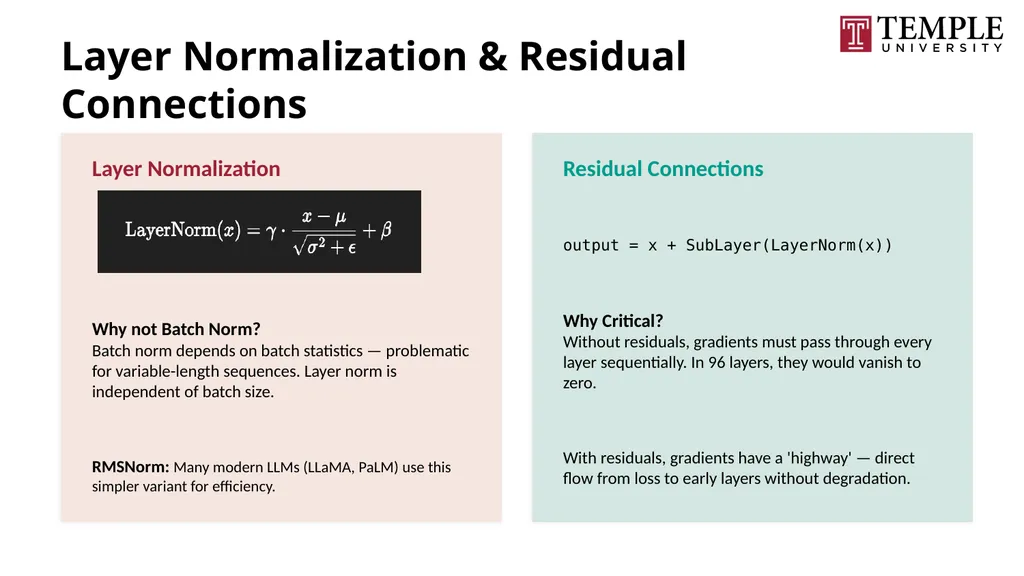
Layer Normalization & Residual Connections Layer Normalization
Why not Batch Norm?
Batch norm depends on batch statistics — problematic for variable-length sequences. Layer norm is independent of batch size.
RMSNorm: Many modern LLMs (LLaMA, PaLM) use this simpler variant for efficiency. Residual Connections
output = x + SubLayer(LayerNorm(x))
Why Critical?
Without residuals, gradients must pass through every layer sequentially. In 96 layers, they would vanish to zero.
With residuals, gradients have a 'highway' — direct flow from loss to early layers without degradation.<br>
Why not Batch Norm?
Batch norm depends on batch statistics — problematic for variable-length sequences. Layer norm is independent of batch size.
RMSNorm: Many modern LLMs (LLaMA, PaLM) use this simpler variant for efficiency. Residual Connections
output = x + SubLayer(LayerNorm(x))
Why Critical?
Without residuals, gradients must pass through every layer sequentially. In 96 layers, they would vanish to zero.
With residuals, gradients have a 'highway' — direct flow from loss to early layers without degradation.<br>
57
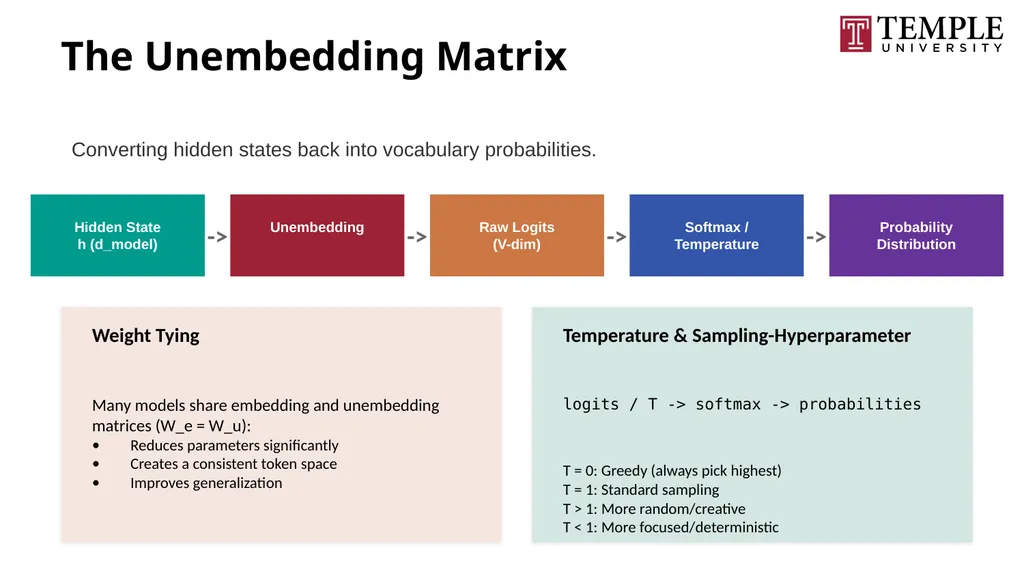
The Unembedding Matrix Converting hidden states back into vocabulary probabilities. Hidden State
h (d_model) -> Unembedding -> Raw Logits
(V-dim) -> Softmax /
Temperature -> Probability
Distribution Weight Tying
Many models share embedding and unembedding matrices (W_e = W_u):
Reduces parameters significantly
Creates a consistent token space
Improves generalization Temperature & Sampling-Hyperparameter
logits / T -> softmax -> probabilities
T = 0: Greedy (always pick highest)
T = 1: Standard sampling
T > 1: More random/creative
T < 1: More focused/deterministic<br>
h (d_model) -> Unembedding -> Raw Logits
(V-dim) -> Softmax /
Temperature -> Probability
Distribution Weight Tying
Many models share embedding and unembedding matrices (W_e = W_u):
Reduces parameters significantly
Creates a consistent token space
Improves generalization Temperature & Sampling-Hyperparameter
logits / T -> softmax -> probabilities
T = 0: Greedy (always pick highest)
T = 1: Standard sampling
T > 1: More random/creative
T < 1: More focused/deterministic<br>
58
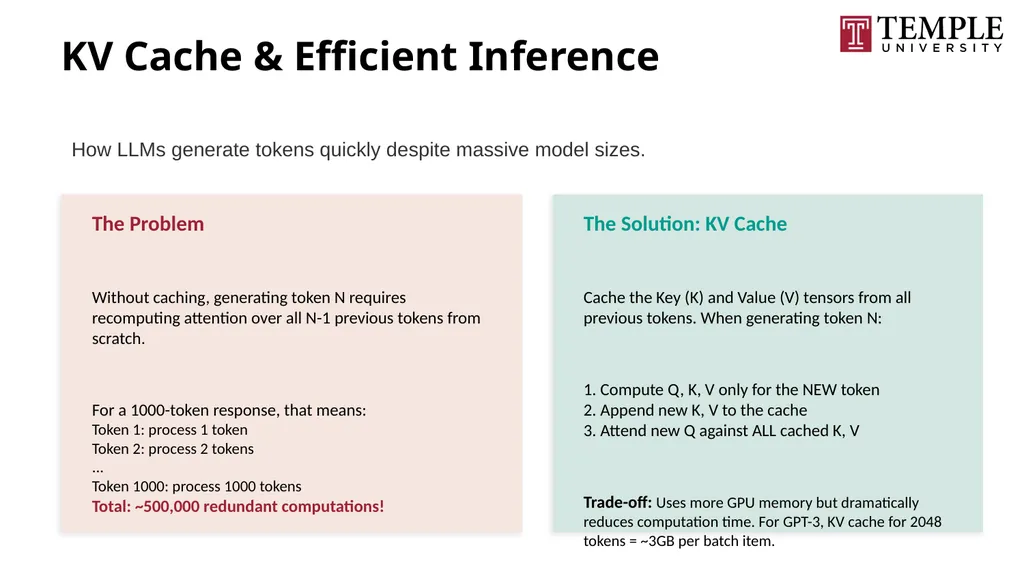
KV Cache & Efficient Inference How LLMs generate tokens quickly despite massive model sizes. The Problem
Without caching, generating token N requires recomputing attention over all N-1 previous tokens from scratch.
For a 1000-token response, that means:
Token 1: process 1 token
Token 2: process 2 tokens
...
Token 1000: process 1000 tokens
Total: ~500,000 redundant computations! The Solution: KV Cache
Cache the Key (K) and Value (V) tensors from all previous tokens. When generating token N:
1. Compute Q, K, V only for the NEW token
2. Append new K, V to the cache
3. Attend new Q against ALL cached K, V
Trade-off: Uses more GPU memory but dramatically reduces computation time. For GPT-3, KV cache for 2048 tokens = ~3GB per batch item.<br>
Without caching, generating token N requires recomputing attention over all N-1 previous tokens from scratch.
For a 1000-token response, that means:
Token 1: process 1 token
Token 2: process 2 tokens
...
Token 1000: process 1000 tokens
Total: ~500,000 redundant computations! The Solution: KV Cache
Cache the Key (K) and Value (V) tensors from all previous tokens. When generating token N:
1. Compute Q, K, V only for the NEW token
2. Append new K, V to the cache
3. Attend new Q against ALL cached K, V
Trade-off: Uses more GPU memory but dramatically reduces computation time. For GPT-3, KV cache for 2048 tokens = ~3GB per batch item.<br>
59
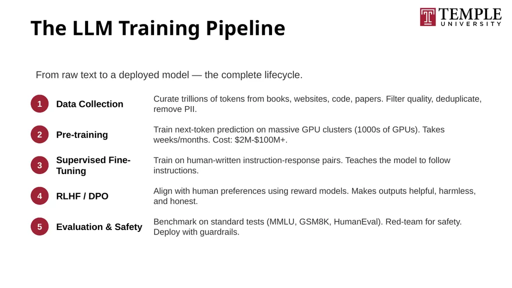
The LLM Training Pipeline From raw text to a deployed model — the complete lifecycle. 1 Data Collection Curate trillions of tokens from books, websites, code, papers. Filter quality, deduplicate, remove PII. 2 Pre-training Train next-token prediction on massive GPU clusters (1000s of GPUs). Takes weeks/months. Cost: $2M-$100M+. 3 Supervised Fine-Tuning Train on human-written instruction-response pairs. Teaches the model to follow instructions. 4 RLHF / DPO Align with human preferences using reward models. Makes outputs helpful, harmless, and honest. 5 Evaluation & Safety Benchmark on standard tests (MMLU, GSM8K, HumanEval). Red-team for safety. Deploy with guardrails.<br>
60
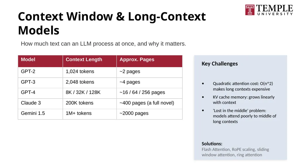
Context Window & Long-Context Models How much text can an LLM process at once, and why it matters. Key Challenges
Quadratic attention cost: O(n^2) makes long contexts expensive
KV cache memory: grows linearly with context
'Lost in the middle' problem: models attend poorly to middle of long contexts
Solutions:
Flash Attention, RoPE scaling, sliding window attention, ring attention<br>
Quadratic attention cost: O(n^2) makes long contexts expensive
KV cache memory: grows linearly with context
'Lost in the middle' problem: models attend poorly to middle of long contexts
Solutions:
Flash Attention, RoPE scaling, sliding window attention, ring attention<br>
61
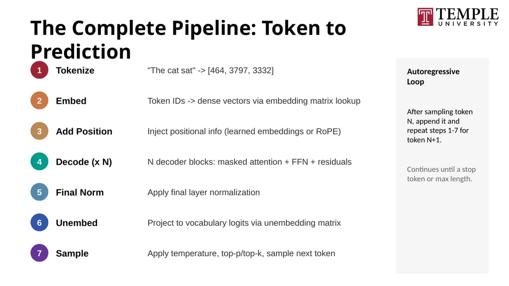
The Complete Pipeline: Token to Prediction 1 Tokenize "The cat sat" -> [464, 3797, 3332] 2 Embed Token IDs -> dense vectors via embedding matrix lookup 3 Add Position Inject positional info (learned embeddings or RoPE) 4 Decode (x N) N decoder blocks: masked attention + FFN + residuals 5 Final Norm Apply final layer normalization 6 Unembed Project to vocabulary logits via unembedding matrix 7 Sample Apply temperature, top-p/top-k, sample next token Autoregressive Loop
After sampling token N, append it and repeat steps 1-7 for token N+1.
Continues until a stop token or max length.<br>
After sampling token N, append it and repeat steps 1-7 for token N+1.
Continues until a stop token or max length.<br>
62
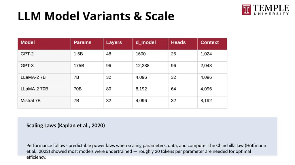
LLM Model Variants & Scale Scaling Laws (Kaplan et al., 2020)
Performance follows predictable power laws when scaling parameters, data, and compute. The Chinchilla law (Hoffmann et al., 2022) showed most models were undertrained — roughly 20 tokens per parameter are needed for optimal efficiency.<br>
Performance follows predictable power laws when scaling parameters, data, and compute. The Chinchilla law (Hoffmann et al., 2022) showed most models were undertrained — roughly 20 tokens per parameter are needed for optimal efficiency.<br>
63
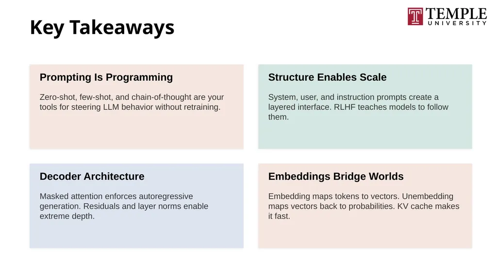
Key Takeaways Prompting Is Programming Zero-shot, few-shot, and chain-of-thought are your tools for steering LLM behavior without retraining. Structure Enables Scale System, user, and instruction prompts create a layered interface. RLHF teaches models to follow them. Decoder Architecture Masked attention enforces autoregressive generation. Residuals and layer norms enable extreme depth. Embeddings Bridge Worlds Embedding maps tokens to vectors. Unembedding maps vectors back to probabilities. KV cache makes it fast.<br>
64
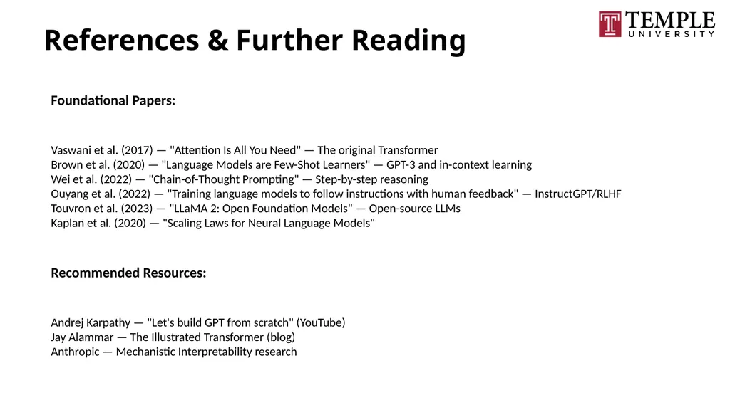
References & Further Reading Foundational Papers:
Vaswani et al. (2017) — "Attention Is All You Need" — The original Transformer
Brown et al. (2020) — "Language Models are Few-Shot Learners" — GPT-3 and in-context learning
Wei et al. (2022) — "Chain-of-Thought Prompting" — Step-by-step reasoning
Ouyang et al. (2022) — "Training language models to follow instructions with human feedback" — InstructGPT/RLHF
Touvron et al. (2023) — "LLaMA 2: Open Foundation Models" — Open-source LLMs
Kaplan et al. (2020) — "Scaling Laws for Neural Language Models"
Recommended Resources:
Andrej Karpathy — "Let's build GPT from scratch" (YouTube)
Jay Alammar — The Illustrated Transformer (blog)
Anthropic — Mechanistic Interpretability research<br>
Vaswani et al. (2017) — "Attention Is All You Need" — The original Transformer
Brown et al. (2020) — "Language Models are Few-Shot Learners" — GPT-3 and in-context learning
Wei et al. (2022) — "Chain-of-Thought Prompting" — Step-by-step reasoning
Ouyang et al. (2022) — "Training language models to follow instructions with human feedback" — InstructGPT/RLHF
Touvron et al. (2023) — "LLaMA 2: Open Foundation Models" — Open-source LLMs
Kaplan et al. (2020) — "Scaling Laws for Neural Language Models"
Recommended Resources:
Andrej Karpathy — "Let's build GPT from scratch" (YouTube)
Jay Alammar — The Illustrated Transformer (blog)
Anthropic — Mechanistic Interpretability research<br>
65
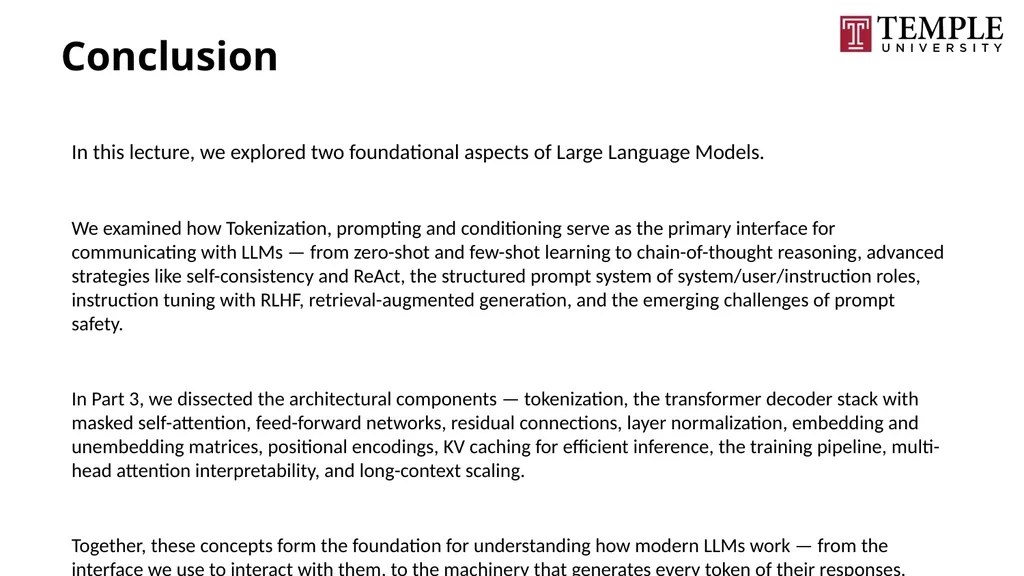
Conclusion In this lecture, we explored two foundational aspects of Large Language Models.
We examined how Tokenization, prompting and conditioning serve as the primary interface for communicating with LLMs — from zero-shot and few-shot learning to chain-of-thought reasoning, advanced strategies like self-consistency and ReAct, the structured prompt system of system/user/instruction roles, instruction tuning with RLHF, retrieval-augmented generation, and the emerging challenges of prompt safety.
In Part 3, we dissected the architectural components — tokenization, the transformer decoder stack with masked self-attention, feed-forward networks, residual connections, layer normalization, embedding and unembedding matrices, positional encodings, KV caching for efficient inference, the training pipeline, multi-head attention interpretability, and long-context scaling.
Together, these concepts form the foundation for understanding how modern LLMs work — from the interface we use to interact with them, to the machinery that generates every token of their responses.<br>
We examined how Tokenization, prompting and conditioning serve as the primary interface for communicating with LLMs — from zero-shot and few-shot learning to chain-of-thought reasoning, advanced strategies like self-consistency and ReAct, the structured prompt system of system/user/instruction roles, instruction tuning with RLHF, retrieval-augmented generation, and the emerging challenges of prompt safety.
In Part 3, we dissected the architectural components — tokenization, the transformer decoder stack with masked self-attention, feed-forward networks, residual connections, layer normalization, embedding and unembedding matrices, positional encodings, KV caching for efficient inference, the training pipeline, multi-head attention interpretability, and long-context scaling.
Together, these concepts form the foundation for understanding how modern LLMs work — from the interface we use to interact with them, to the machinery that generates every token of their responses.<br>