
What is Data? An attribute is a property or
Description: What is Data? An attribute is a property or characteristic of an object Examples: eye color of a person, temperature, etc. An Attribute is also known as variable, field, characteristic, or feature A collection of attributes describe an
Related Topics
Download Presentation
"What is Data? An attribute is a property or" is the property of its rightful owner. Permission is granted to download and print the materials on this website for personal, non-commercial use only, and to display it on your personal computer provided you do not modify the materials and that you retain all copyright notices contained in the materials. By downloading content from our website, you accept the terms of this agreement.
Presentation Transcript
slide1. What is Data?
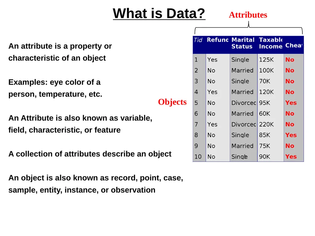
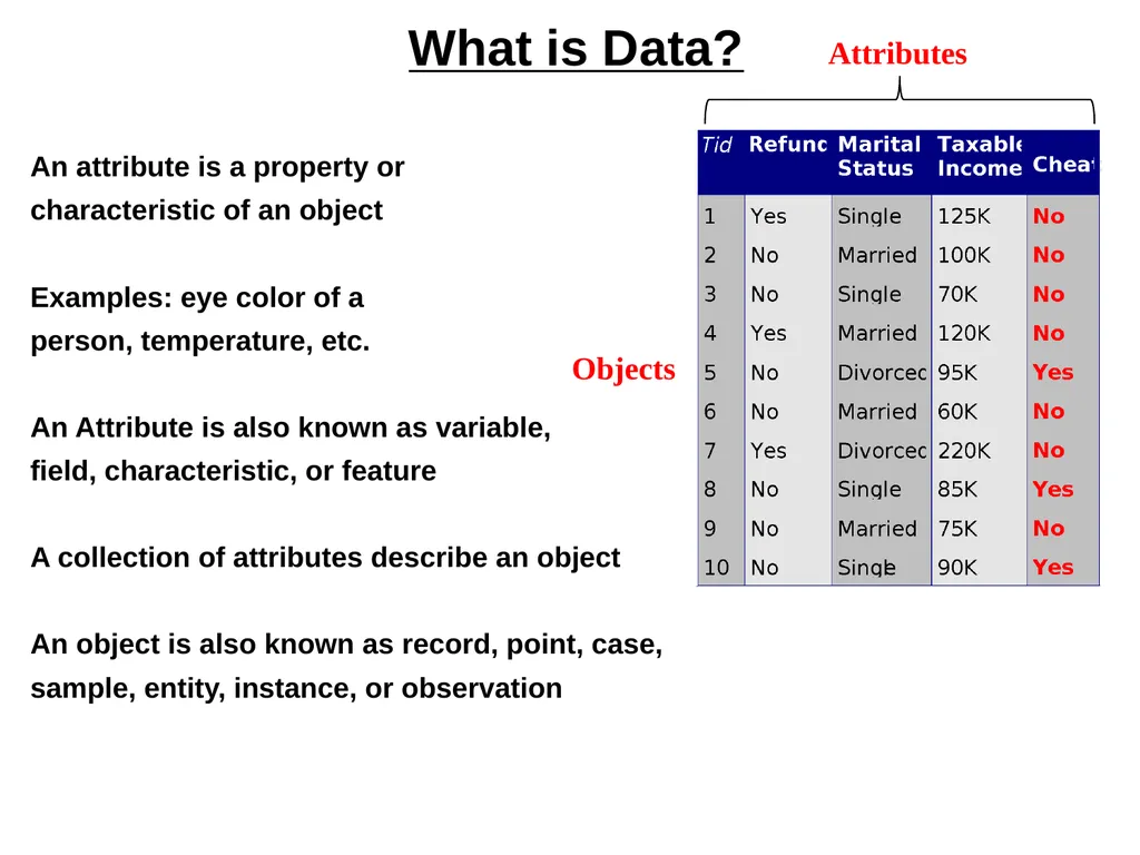
An attribute is a property or
characteristic of an object
Examples: eye color of a
person, temperature, etc.
An Attribute is also known as variable,
field, characteristic, or feature
A collection of attributes describe an object
An object is also known as record, point, case,
sample, entity, instance, or observation Attributes Objects<br>
slide2. Experimental vs. Observational Data
(Important but not in book)
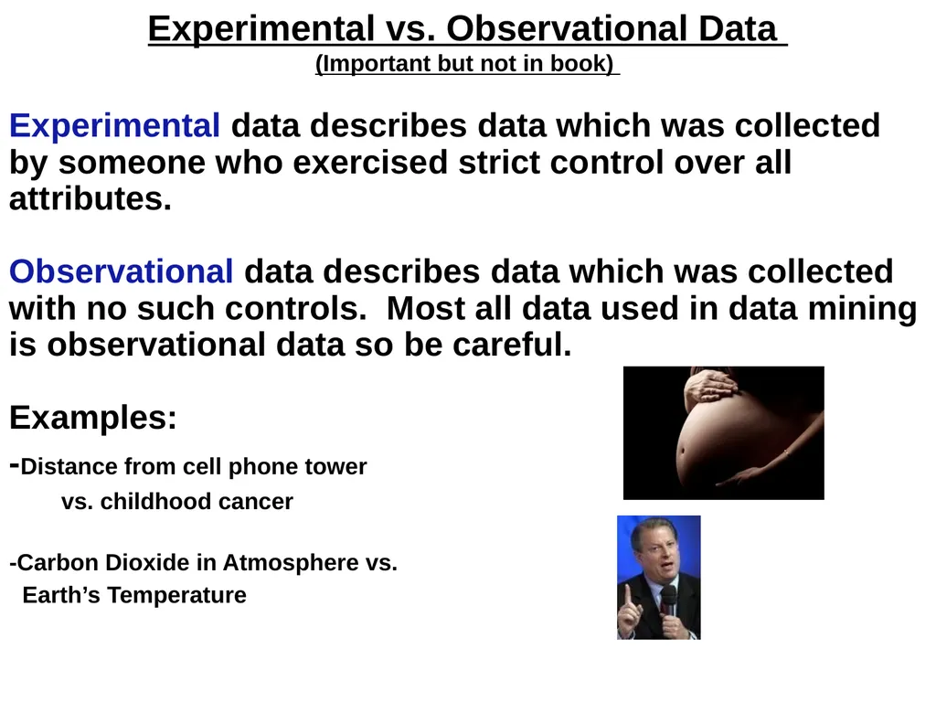
Experimental data describes data which was collected by someone who exercised strict control over all attributes.
Observational data describes data which was collected with no such controls. Most all data used in data mining is observational data so be careful.
Examples:
-Distance from cell phone tower
vs. childhood cancer
-Carbon Dioxide in Atmosphere vs.
Earth’s Temperature<br>
slide3. Types of Attributes:
Qualitative vs. Quantitative (P. 26)
Qualitative (or Categorical) attributes represent distinct categories rather than numbers. Mathematical operations such as addition and subtraction do not make sense. Examples:
eye color, letter grade, IP address, zip code
Quantitative (or Numeric) attributes are numbers and can be treated as such. Examples:
weight, failures per hour, number of TVs, temperature<br>
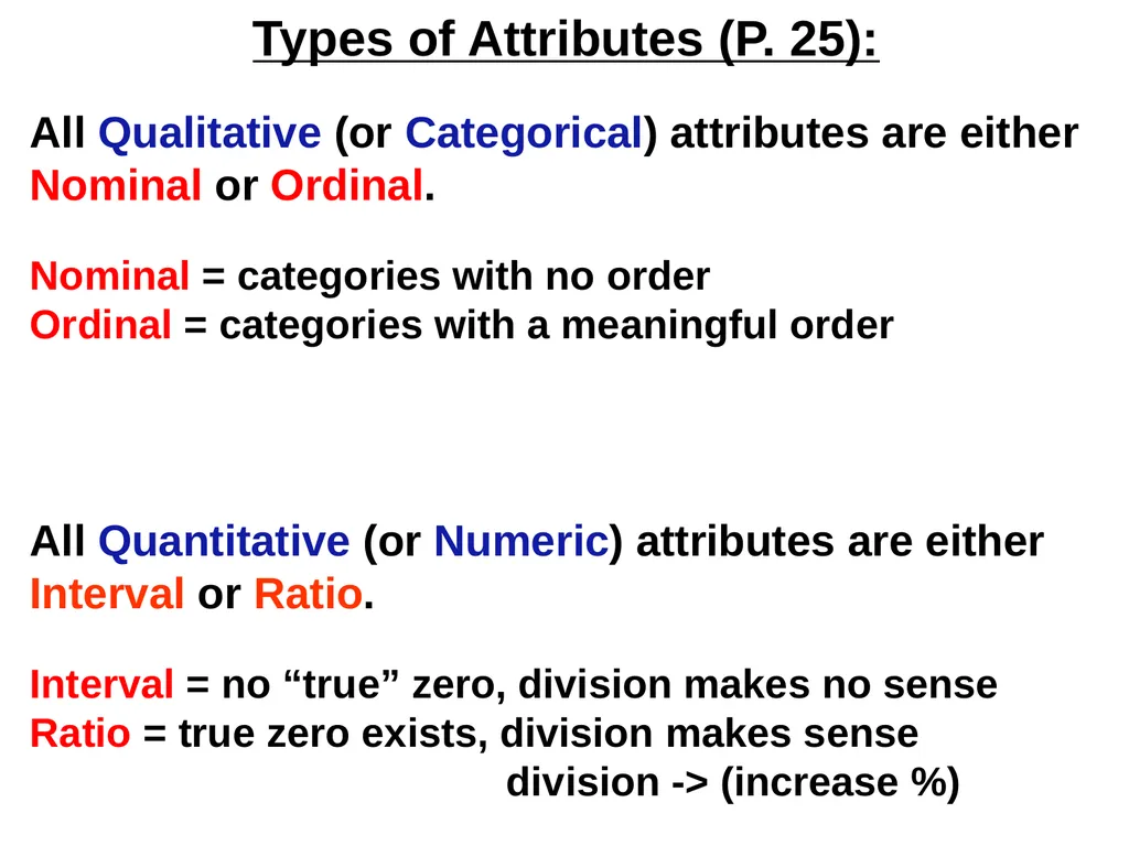
slide4. Types of Attributes (P. 25):
All Qualitative (or Categorical) attributes are either Nominal or Ordinal.
Nominal = categories with no order
Ordinal = categories with a meaningful order
All Quantitative (or Numeric) attributes are either Interval or Ratio.
Interval = no “true” zero, division makes no sense
Ratio = true zero exists, division makes sense
division -> (increase %)<br>
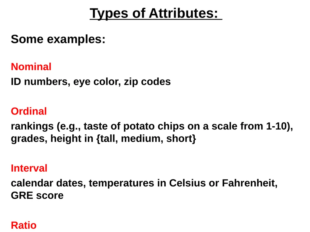
slide5. Types of Attributes:
Some examples:
Nominal
ID numbers, eye color, zip codes
Ordinal
rankings (e.g., taste of potato chips on a scale from 1-10), grades, height in {tall, medium, short}
Interval
calendar dates, temperatures in Celsius or Fahrenheit, GRE score
Ratio
temperature in Kelvin, length, time, counts<br>
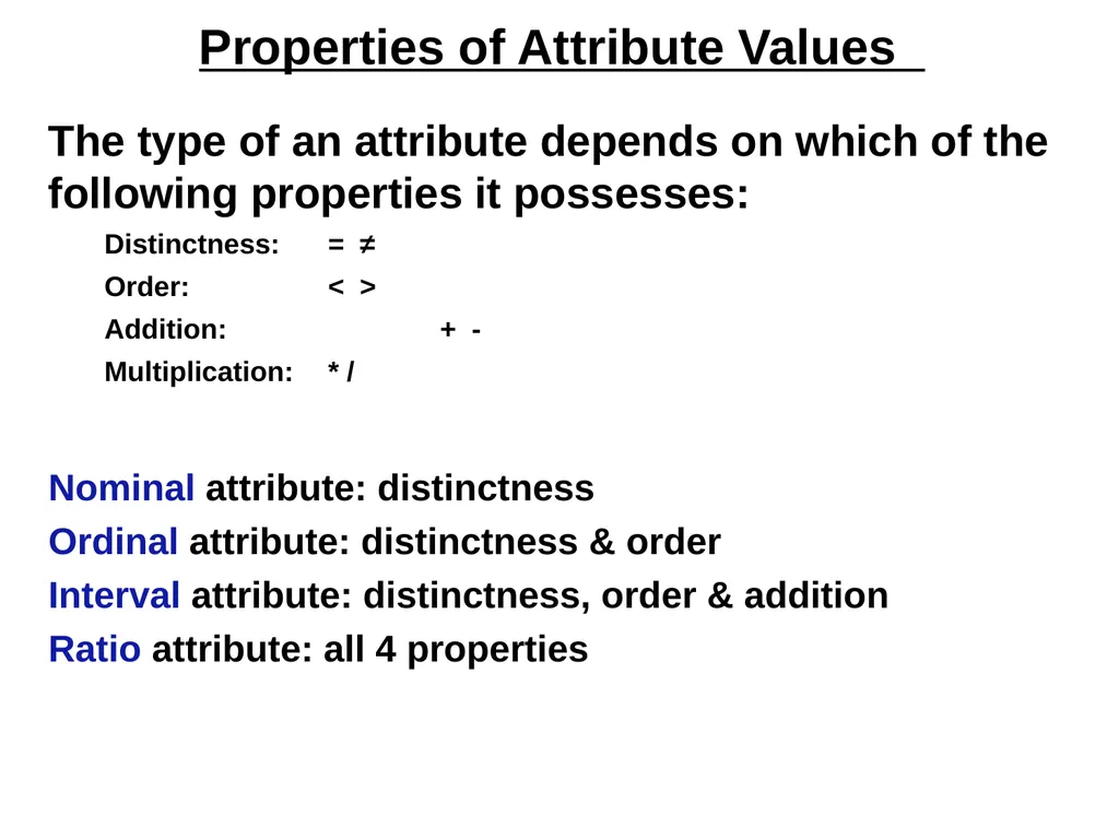
slide6. Properties of Attribute Values
The type of an attribute depends on which of the following properties it possesses:
Distinctness: = ≠
Order: < >
Addition: + -
Multiplication: * /
Nominal attribute: distinctness
Ordinal attribute: distinctness & order
Interval attribute: distinctness, order & addition
Ratio attribute: all 4 properties<br>
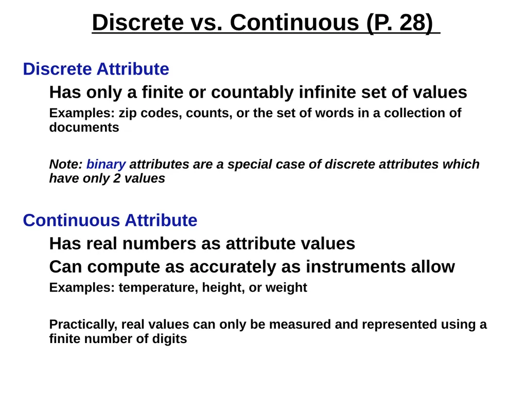
slide7. Discrete vs. Continuous (P. 28)
Discrete Attribute
Has only a finite or countably infinite set of values
Examples: zip codes, counts, or the set of words in a collection of documents
Note: binary attributes are a special case of discrete attributes which have only 2 values
Continuous Attribute
Has real numbers as attribute values
Can compute as accurately as instruments allow
Examples: temperature, height, or weight
Practically, real values can only be measured and represented using a finite number of digits<br>
slide8. Discrete vs. Continuous (P. 28)
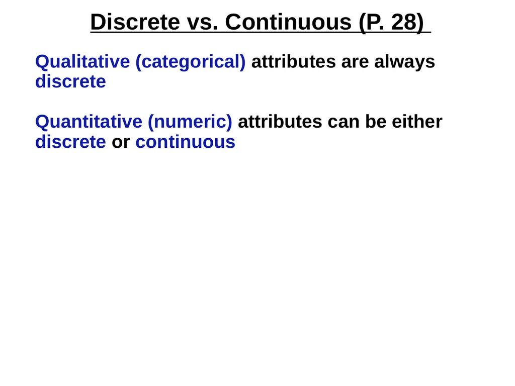
Qualitative (categorical) attributes are always discrete
Quantitative (numeric) attributes can be either discrete or continuous<br>
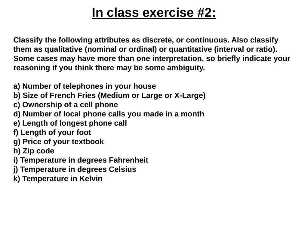
slide9. In class exercise #2:
Classify the following attributes as discrete, or continuous. Also classify them as qualitative (nominal or ordinal) or quantitative (interval or ratio). Some cases may have more than one interpretation, so briefly indicate your reasoning if you think there may be some ambiguity.
a) Number of telephones in your house
b) Size of French Fries (Medium or Large or X-Large)
c) Ownership of a cell phone
d) Number of local phone calls you made in a month
e) Length of longest phone call
f) Length of your foot
g) Price of your textbook
h) Zip code
i) Temperature in degrees Fahrenheit
j) Temperature in degrees Celsius
k) Temperature in Kelvin<br>
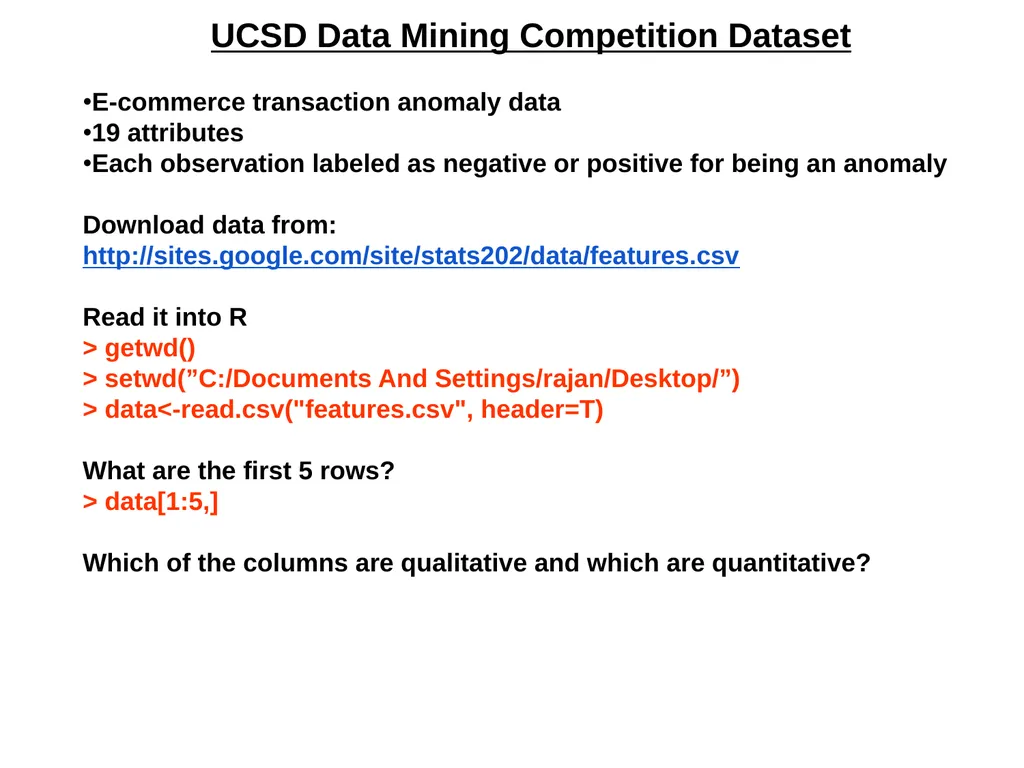
slide10. UCSD Data Mining Competition Dataset
E-commerce transaction anomaly data
19 attributes
Each observation labeled as negative or positive for being an anomaly
Download data from:
http://sites.google.com/site/stats202/data/features.csv
Read it into R
> getwd()
> setwd(”C:/Documents And Settings/rajan/Desktop/”)
> data<-read.csv("features.csv", header=T)
What are the first 5 rows?
> data[1:5,]
Which of the columns are qualitative and which are quantitative?<br>
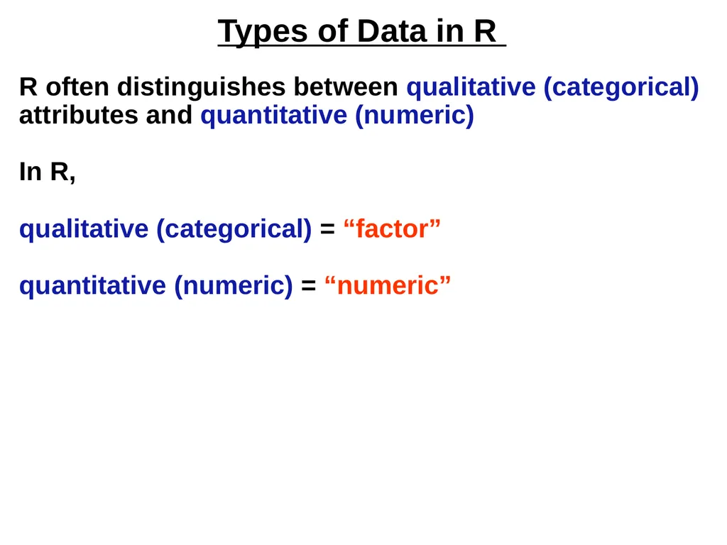
slide11. Types of Data in R
R often distinguishes between qualitative (categorical) attributes and quantitative (numeric)
In R,
qualitative (categorical) = “factor”
quantitative (numeric) = “numeric”<br>
slide12. Types of Data in R
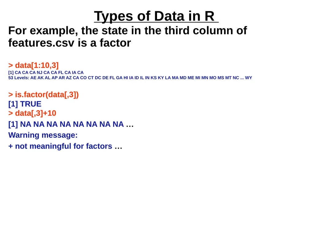
For example, the state in the third column of features.csv is a factor
> data[1:10,3]
[1] CA CA CA NJ CA CA FL CA IA CA
53 Levels: AE AK AL AP AR AZ CA CO CT DC DE FL GA HI IA ID IL IN KS KY LA MA MD ME MI MN MO MS MT NC ... WY
> is.factor(data[,3])
[1] TRUE
> data[,3]+10
[1] NA NA NA NA NA NA NA NA …
Warning message:
+ not meaningful for factors …<br>
slide13. Types of Data in R
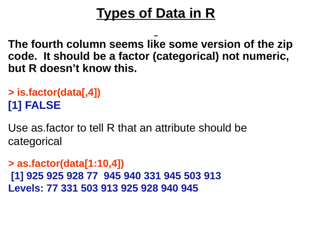
The fourth column seems like some version of the zip code. It should be a factor (categorical) not numeric, but R doesn’t know this.
> is.factor(data[,4])
[1] FALSE
Use as.factor to tell R that an attribute should be categorical
> as.factor(data[1:10,4])
[1] 925 925 928 77 945 940 331 945 503 913
Levels: 77 331 503 913 925 928 940 945<br>
slide14. Working with Data in R
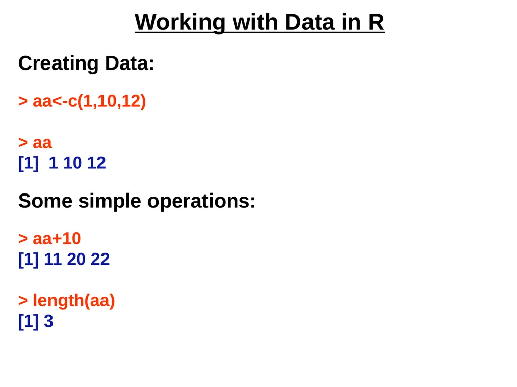
Creating Data:
> aa<-c(1,10,12)
> aa
[1] 1 10 12
Some simple operations:
> aa+10
[1] 11 20 22
> length(aa)
[1] 3<br>
slide15. Working with Data in R
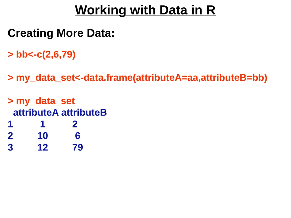
Creating More Data:
> bb<-c(2,6,79)
> my_data_set<-data.frame(attributeA=aa,attributeB=bb)
> my_data_set
attributeA attributeB
1 1 2
2 10 6
3 12 79<br>
slide16. Working with Data in R
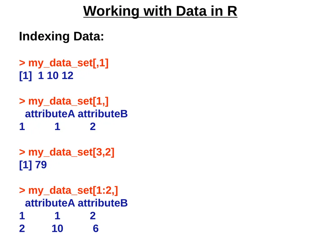
Indexing Data:
> my_data_set[,1]
[1] 1 10 12
> my_data_set[1,]
attributeA attributeB
1 1 2
> my_data_set[3,2]
[1] 79
> my_data_set[1:2,]
attributeA attributeB
1 1 2
2 10 6<br>
slide17. Working with Data in R
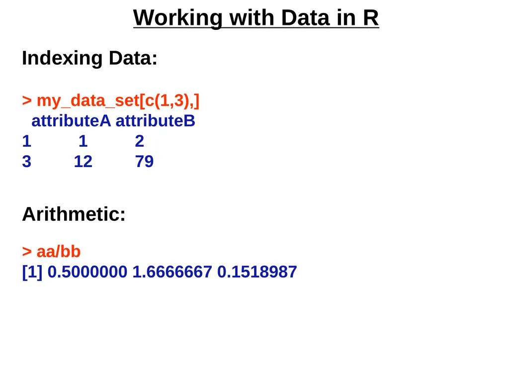
Indexing Data:
> my_data_set[c(1,3),]
attributeA attributeB
1 1 2
3 12 79
Arithmetic:
> aa/bb
[1] 0.5000000 1.6666667 0.1518987<br>
slide18. Working with Data in R
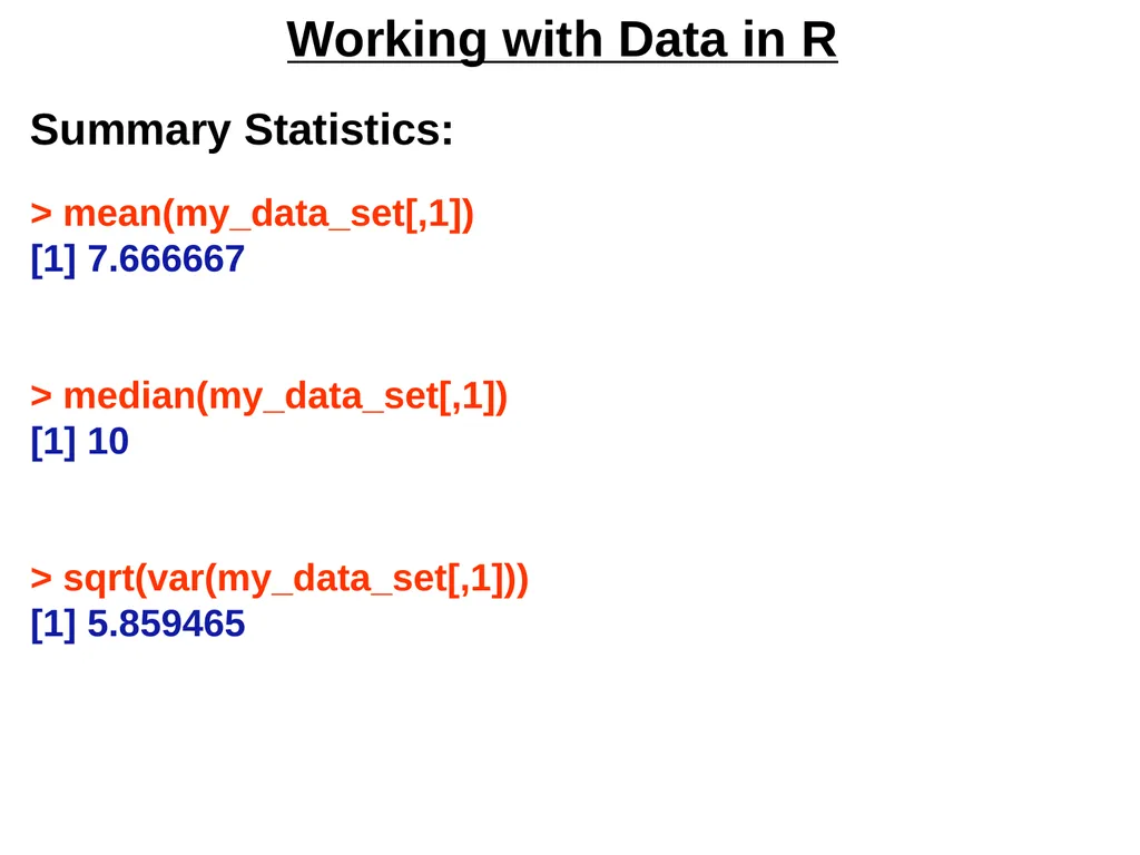
Summary Statistics:
> mean(my_data_set[,1])
[1] 7.666667
> median(my_data_set[,1])
[1] 10
> sqrt(var(my_data_set[,1]))
[1] 5.859465<br>
slide19. * Working with Data in R
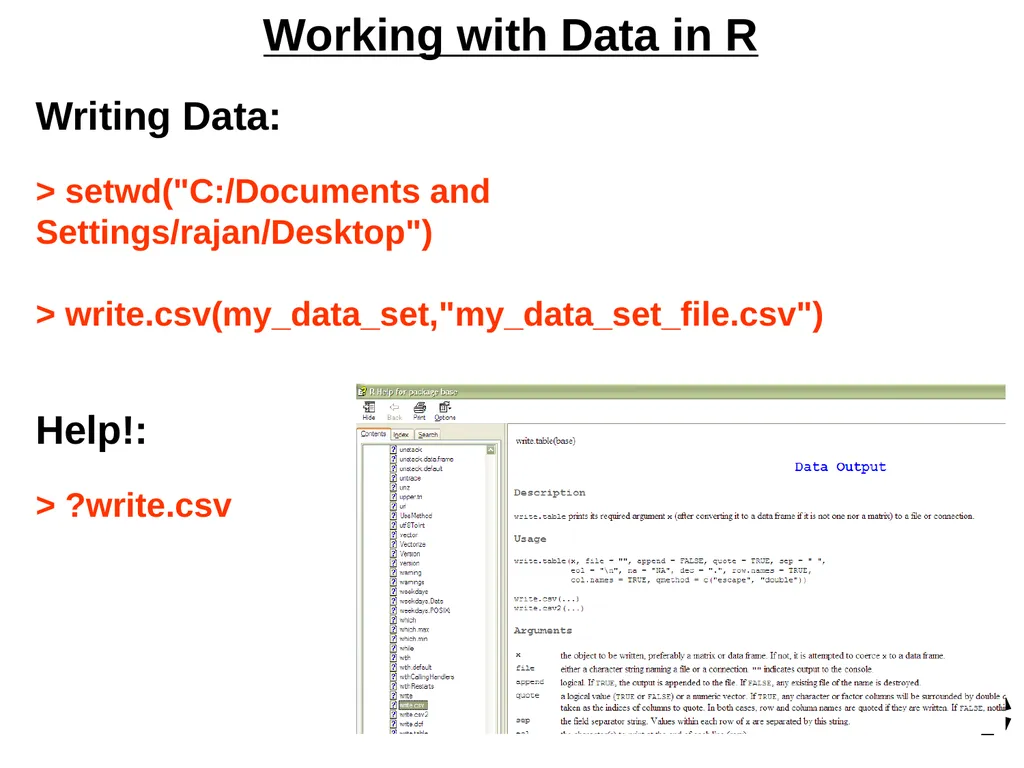
Writing Data:
> setwd("C:/Documents and
Settings/rajan/Desktop")
> write.csv(my_data_set,"my_data_set_file.csv")
Help!:
> ?write.csv<br>
slide20. Sampling
Sampling involves using only a random subset of the data for analysis
Statisticians are interested in sampling because they often can not get all the data from a population of interest
Data miners are interested in sampling because sometimes using all the data they have is too slow and unnecessary<br>
slide21. Sampling
The key principle for effective sampling is the following:
using a sample will work almost as well as using the entire data sets, if the sample is representative
a sample is representative if it has approximately the same property (of interest) as the original set of data<br>
slide22. Sampling
The simple random sample is the most common and basic type of sample
In a simple random sample every item has the same probability of inclusion and every sample of the fixed size has the same probability of selection
It is the standard “names out of a hat”
It can be with replacement (=items can be chosen more than once) or without replacement (=items can be chosen only once)
More complex schemes exist (examples: stratified sampling, cluster sampling)<br>
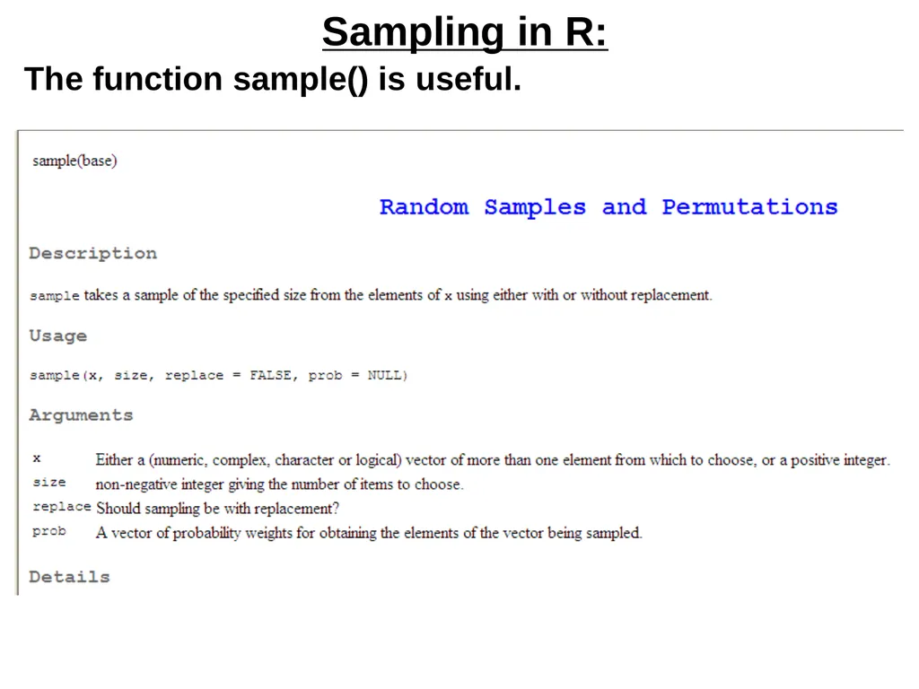
slide23. Sampling in R:
The function sample() is useful.<br>
slide24. In class exercise #3:
Explain how to use R to draw a sample of 10 observations with replacement from the first quantitative attribute in the data set http://sites.google.com/site/stats202/data/features.csv<br>
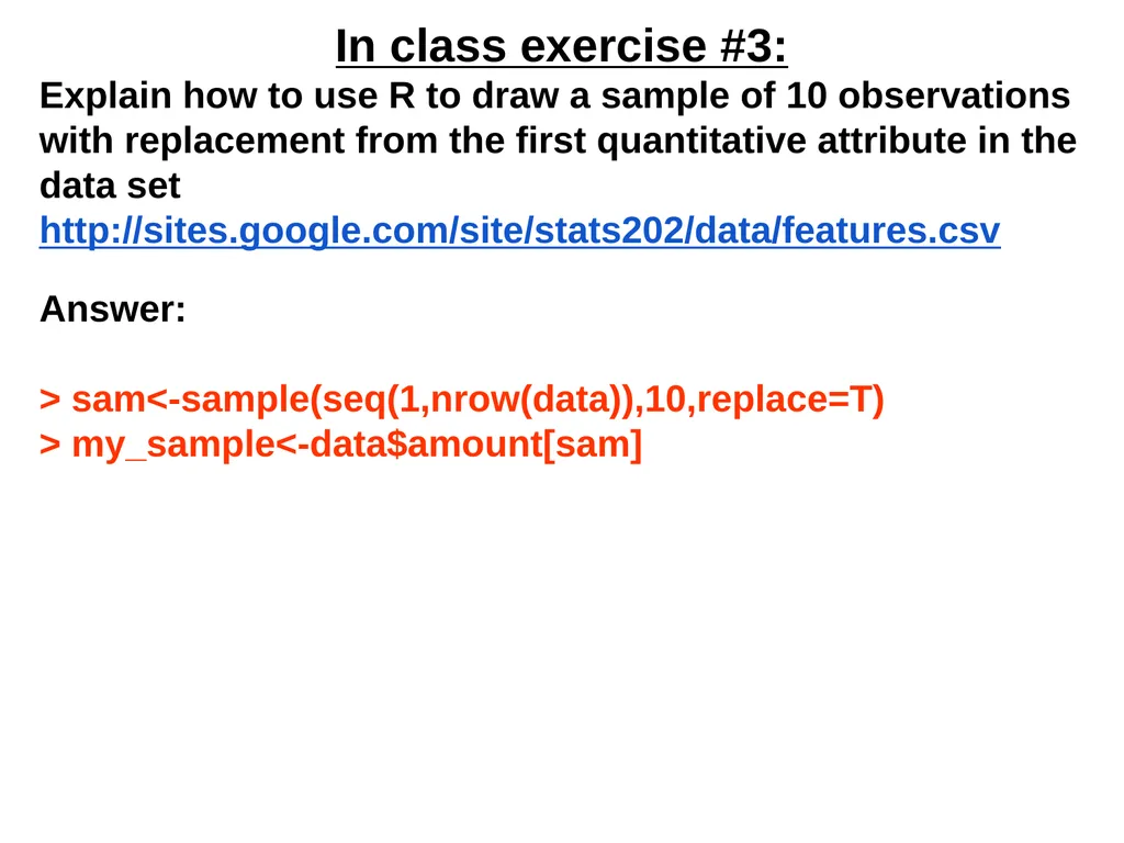
slide25. In class exercise #3:
Explain how to use R to draw a sample of 10 observations with replacement from the first quantitative attribute in the data set http://sites.google.com/site/stats202/data/features.csv
Answer:
> sam<-sample(seq(1,nrow(data)),10,replace=T)
> my_sample<-data$amount[sam]<br>
slide26. In class exercise #4:
If you do the sampling in the previous exercise repeatedly, roughly how far is the mean of the sample from the mean of the whole column on average?<br>
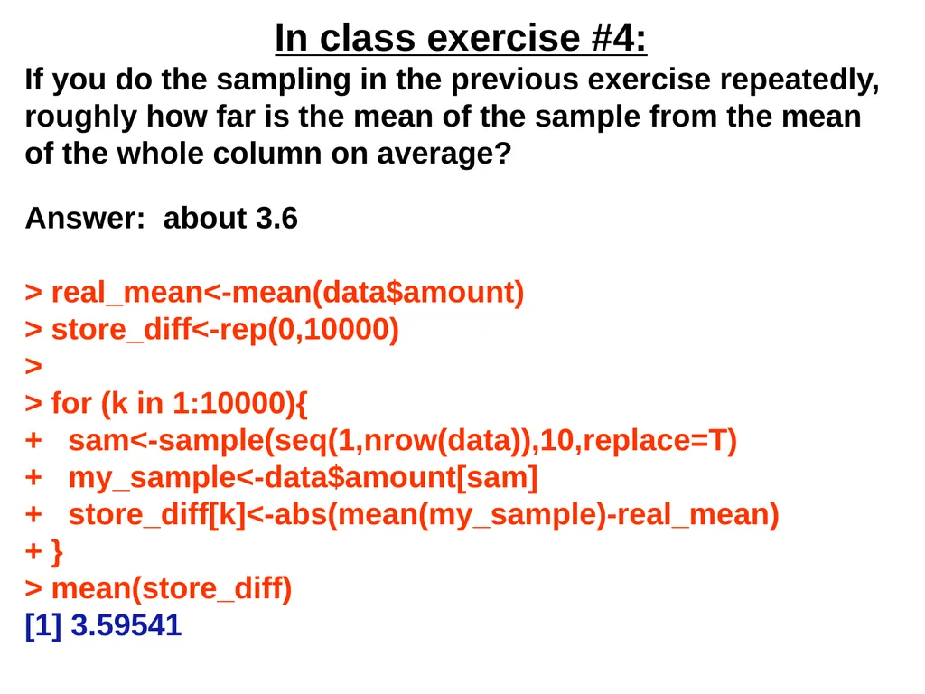
slide27. In class exercise #4:
If you do the sampling in the previous exercise repeatedly, roughly how far is the mean of the sample from the mean of the whole column on average?
Answer: about 3.6
> real_mean<-mean(data$amount)
> store_diff<-rep(0,10000)
>
> for (k in 1:10000){
+ sam<-sample(seq(1,nrow(data)),10,replace=T)
+ my_sample<-data$amount[sam]
+ store_diff[k]<-abs(mean(my_sample)-real_mean)
+ }
> mean(store_diff)
[1] 3.59541<br>
slide28. In class exercise #5:
If you change the sample size from 10 to 100, how does your answer to the previous question change?<br>
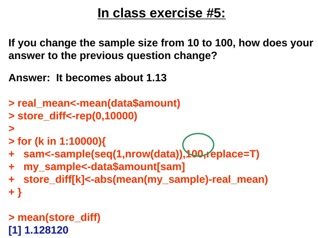
slide29. In class exercise #5:
If you change the sample size from 10 to 100, how does your answer to the previous question change?
Answer: It becomes about 1.13
> real_mean<-mean(data$amount)
> store_diff<-rep(0,10000)
>
> for (k in 1:10000){
+ sam<-sample(seq(1,nrow(data)),100,replace=T)
+ my_sample<-data$amount[sam]
+ store_diff[k]<-abs(mean(my_sample)-real_mean)
+ }
> mean(store_diff)
[1] 1.128120<br>
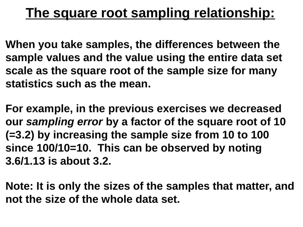
slide30. The square root sampling relationship:
When you take samples, the differences between the sample values and the value using the entire data set scale as the square root of the sample size for many statistics such as the mean.
For example, in the previous exercises we decreased our sampling error by a factor of the square root of 10 (=3.2) by increasing the sample size from 10 to 100 since 100/10=10. This can be observed by noting 3.6/1.13 is about 3.2.
Note: It is only the sizes of the samples that matter, and not the size of the whole data set.<br>
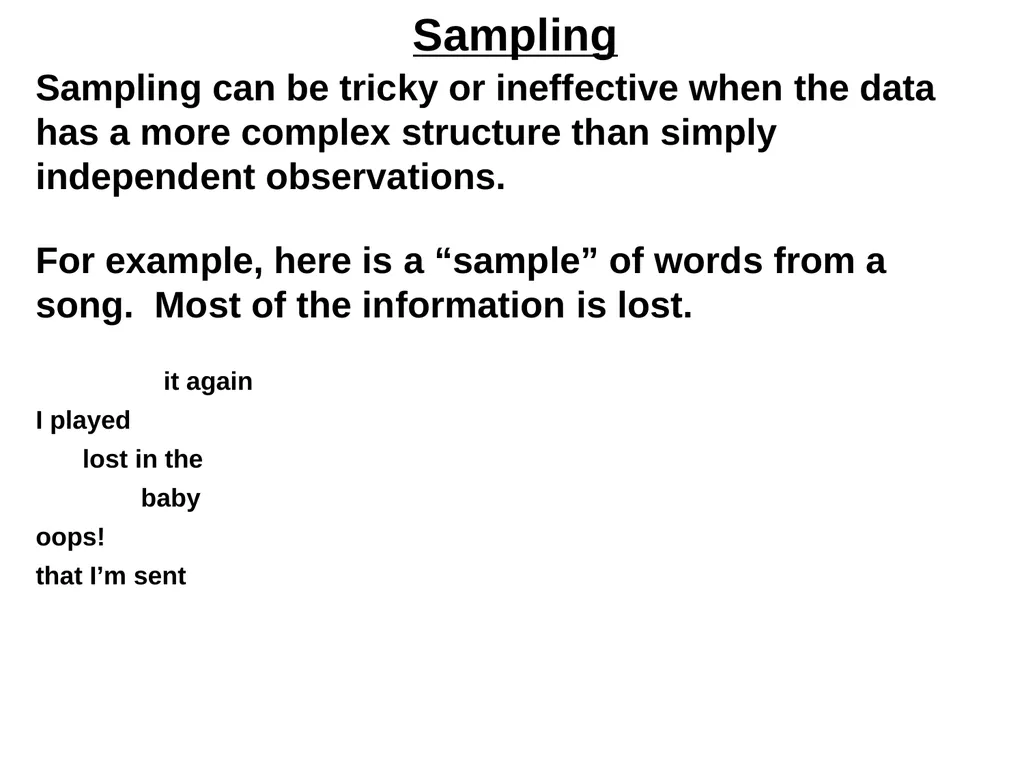
slide31. Sampling
Sampling can be tricky or ineffective when the data has a more complex structure than simply independent observations.
For example, here is a “sample” of words from a song. Most of the information is lost.
oops I did it again
I played with your heart
got lost in the game
oh baby baby
oops! ...you think I’m in love
that I’m sent from above
I’m not that innocent<br>
slide32. Sampling
Sampling can be tricky or ineffective when the data has a more complex structure than simply independent observations.
For example, here is a “sample” of words from a song. Most of the information is lost.
oops I did it again
I played with your heart
got lost in the game
oh baby baby
oops! ...you think I’m in love
that I’m sent from above
I’m not that innocent<br>
An attribute is a property or
characteristic of an object
Examples: eye color of a
person, temperature, etc.
An Attribute is also known as variable,
field, characteristic, or feature
A collection of attributes describe an object
An object is also known as record, point, case,
sample, entity, instance, or observation Attributes Objects<br>
slide2. Experimental vs. Observational Data
(Important but not in book)
Experimental data describes data which was collected by someone who exercised strict control over all attributes.
Observational data describes data which was collected with no such controls. Most all data used in data mining is observational data so be careful.
Examples:
-Distance from cell phone tower
vs. childhood cancer
-Carbon Dioxide in Atmosphere vs.
Earth’s Temperature<br>
slide3. Types of Attributes:
Qualitative vs. Quantitative (P. 26)
Qualitative (or Categorical) attributes represent distinct categories rather than numbers. Mathematical operations such as addition and subtraction do not make sense. Examples:
eye color, letter grade, IP address, zip code
Quantitative (or Numeric) attributes are numbers and can be treated as such. Examples:
weight, failures per hour, number of TVs, temperature<br>
slide4. Types of Attributes (P. 25):
All Qualitative (or Categorical) attributes are either Nominal or Ordinal.
Nominal = categories with no order
Ordinal = categories with a meaningful order
All Quantitative (or Numeric) attributes are either Interval or Ratio.
Interval = no “true” zero, division makes no sense
Ratio = true zero exists, division makes sense
division -> (increase %)<br>
slide5. Types of Attributes:
Some examples:
Nominal
ID numbers, eye color, zip codes
Ordinal
rankings (e.g., taste of potato chips on a scale from 1-10), grades, height in {tall, medium, short}
Interval
calendar dates, temperatures in Celsius or Fahrenheit, GRE score
Ratio
temperature in Kelvin, length, time, counts<br>
slide6. Properties of Attribute Values
The type of an attribute depends on which of the following properties it possesses:
Distinctness: = ≠
Order: < >
Addition: + -
Multiplication: * /
Nominal attribute: distinctness
Ordinal attribute: distinctness & order
Interval attribute: distinctness, order & addition
Ratio attribute: all 4 properties<br>
slide7. Discrete vs. Continuous (P. 28)
Discrete Attribute
Has only a finite or countably infinite set of values
Examples: zip codes, counts, or the set of words in a collection of documents
Note: binary attributes are a special case of discrete attributes which have only 2 values
Continuous Attribute
Has real numbers as attribute values
Can compute as accurately as instruments allow
Examples: temperature, height, or weight
Practically, real values can only be measured and represented using a finite number of digits<br>
slide8. Discrete vs. Continuous (P. 28)
Qualitative (categorical) attributes are always discrete
Quantitative (numeric) attributes can be either discrete or continuous<br>
slide9. In class exercise #2:
Classify the following attributes as discrete, or continuous. Also classify them as qualitative (nominal or ordinal) or quantitative (interval or ratio). Some cases may have more than one interpretation, so briefly indicate your reasoning if you think there may be some ambiguity.
a) Number of telephones in your house
b) Size of French Fries (Medium or Large or X-Large)
c) Ownership of a cell phone
d) Number of local phone calls you made in a month
e) Length of longest phone call
f) Length of your foot
g) Price of your textbook
h) Zip code
i) Temperature in degrees Fahrenheit
j) Temperature in degrees Celsius
k) Temperature in Kelvin<br>
slide10. UCSD Data Mining Competition Dataset
E-commerce transaction anomaly data
19 attributes
Each observation labeled as negative or positive for being an anomaly
Download data from:
http://sites.google.com/site/stats202/data/features.csv
Read it into R
> getwd()
> setwd(”C:/Documents And Settings/rajan/Desktop/”)
> data<-read.csv("features.csv", header=T)
What are the first 5 rows?
> data[1:5,]
Which of the columns are qualitative and which are quantitative?<br>
slide11. Types of Data in R
R often distinguishes between qualitative (categorical) attributes and quantitative (numeric)
In R,
qualitative (categorical) = “factor”
quantitative (numeric) = “numeric”<br>
slide12. Types of Data in R
For example, the state in the third column of features.csv is a factor
> data[1:10,3]
[1] CA CA CA NJ CA CA FL CA IA CA
53 Levels: AE AK AL AP AR AZ CA CO CT DC DE FL GA HI IA ID IL IN KS KY LA MA MD ME MI MN MO MS MT NC ... WY
> is.factor(data[,3])
[1] TRUE
> data[,3]+10
[1] NA NA NA NA NA NA NA NA …
Warning message:
+ not meaningful for factors …<br>
slide13. Types of Data in R
The fourth column seems like some version of the zip code. It should be a factor (categorical) not numeric, but R doesn’t know this.
> is.factor(data[,4])
[1] FALSE
Use as.factor to tell R that an attribute should be categorical
> as.factor(data[1:10,4])
[1] 925 925 928 77 945 940 331 945 503 913
Levels: 77 331 503 913 925 928 940 945<br>
slide14. Working with Data in R
Creating Data:
> aa<-c(1,10,12)
> aa
[1] 1 10 12
Some simple operations:
> aa+10
[1] 11 20 22
> length(aa)
[1] 3<br>
slide15. Working with Data in R
Creating More Data:
> bb<-c(2,6,79)
> my_data_set<-data.frame(attributeA=aa,attributeB=bb)
> my_data_set
attributeA attributeB
1 1 2
2 10 6
3 12 79<br>
slide16. Working with Data in R
Indexing Data:
> my_data_set[,1]
[1] 1 10 12
> my_data_set[1,]
attributeA attributeB
1 1 2
> my_data_set[3,2]
[1] 79
> my_data_set[1:2,]
attributeA attributeB
1 1 2
2 10 6<br>
slide17. Working with Data in R
Indexing Data:
> my_data_set[c(1,3),]
attributeA attributeB
1 1 2
3 12 79
Arithmetic:
> aa/bb
[1] 0.5000000 1.6666667 0.1518987<br>
slide18. Working with Data in R
Summary Statistics:
> mean(my_data_set[,1])
[1] 7.666667
> median(my_data_set[,1])
[1] 10
> sqrt(var(my_data_set[,1]))
[1] 5.859465<br>
slide19. * Working with Data in R
Writing Data:
> setwd("C:/Documents and
Settings/rajan/Desktop")
> write.csv(my_data_set,"my_data_set_file.csv")
Help!:
> ?write.csv<br>
slide20. Sampling
Sampling involves using only a random subset of the data for analysis
Statisticians are interested in sampling because they often can not get all the data from a population of interest
Data miners are interested in sampling because sometimes using all the data they have is too slow and unnecessary<br>
slide21. Sampling
The key principle for effective sampling is the following:
using a sample will work almost as well as using the entire data sets, if the sample is representative
a sample is representative if it has approximately the same property (of interest) as the original set of data<br>
slide22. Sampling
The simple random sample is the most common and basic type of sample
In a simple random sample every item has the same probability of inclusion and every sample of the fixed size has the same probability of selection
It is the standard “names out of a hat”
It can be with replacement (=items can be chosen more than once) or without replacement (=items can be chosen only once)
More complex schemes exist (examples: stratified sampling, cluster sampling)<br>
slide23. Sampling in R:
The function sample() is useful.<br>
slide24. In class exercise #3:
Explain how to use R to draw a sample of 10 observations with replacement from the first quantitative attribute in the data set http://sites.google.com/site/stats202/data/features.csv<br>
slide25. In class exercise #3:
Explain how to use R to draw a sample of 10 observations with replacement from the first quantitative attribute in the data set http://sites.google.com/site/stats202/data/features.csv
Answer:
> sam<-sample(seq(1,nrow(data)),10,replace=T)
> my_sample<-data$amount[sam]<br>
slide26. In class exercise #4:
If you do the sampling in the previous exercise repeatedly, roughly how far is the mean of the sample from the mean of the whole column on average?<br>
slide27. In class exercise #4:
If you do the sampling in the previous exercise repeatedly, roughly how far is the mean of the sample from the mean of the whole column on average?
Answer: about 3.6
> real_mean<-mean(data$amount)
> store_diff<-rep(0,10000)
>
> for (k in 1:10000){
+ sam<-sample(seq(1,nrow(data)),10,replace=T)
+ my_sample<-data$amount[sam]
+ store_diff[k]<-abs(mean(my_sample)-real_mean)
+ }
> mean(store_diff)
[1] 3.59541<br>
slide28. In class exercise #5:
If you change the sample size from 10 to 100, how does your answer to the previous question change?<br>
slide29. In class exercise #5:
If you change the sample size from 10 to 100, how does your answer to the previous question change?
Answer: It becomes about 1.13
> real_mean<-mean(data$amount)
> store_diff<-rep(0,10000)
>
> for (k in 1:10000){
+ sam<-sample(seq(1,nrow(data)),100,replace=T)
+ my_sample<-data$amount[sam]
+ store_diff[k]<-abs(mean(my_sample)-real_mean)
+ }
> mean(store_diff)
[1] 1.128120<br>
slide30. The square root sampling relationship:
When you take samples, the differences between the sample values and the value using the entire data set scale as the square root of the sample size for many statistics such as the mean.
For example, in the previous exercises we decreased our sampling error by a factor of the square root of 10 (=3.2) by increasing the sample size from 10 to 100 since 100/10=10. This can be observed by noting 3.6/1.13 is about 3.2.
Note: It is only the sizes of the samples that matter, and not the size of the whole data set.<br>
slide31. Sampling
Sampling can be tricky or ineffective when the data has a more complex structure than simply independent observations.
For example, here is a “sample” of words from a song. Most of the information is lost.
oops I did it again
I played with your heart
got lost in the game
oh baby baby
oops! ...you think I’m in love
that I’m sent from above
I’m not that innocent<br>
slide32. Sampling
Sampling can be tricky or ineffective when the data has a more complex structure than simply independent observations.
For example, here is a “sample” of words from a song. Most of the information is lost.
oops I did it again
I played with your heart
got lost in the game
oh baby baby
oops! ...you think I’m in love
that I’m sent from above
I’m not that innocent<br>