www.carteeh.org Lecture #11: Traffic Modeling

slide1. www.carteeh.org<br>
slide2. Lecture #11: Traffic Modeling Methods and Data Sources Angshuman Guin, Ph.D.
Senior Research Engineer
School of Civil and Environmental Engineering
Georgia Institute of Technology
Atlanta, GA 30332
(Email: angshuman.guin@ce.gatech.edu Phone: 404.894.5830)
In addition to his academic affiliation, Dr. Guin is a co-founder of InstaData Systems LLC, Roswell GA 30076
The author has no known conflict of interest.

Lecture Track(s): TT<br>
slide3. Introduction A traffic model is a mathematical model of real-world traffic, usually, but not restricted to, road traffic. Traffic modeling draws heavily on theoretical foundations like network theory and certain theories from physics like the kinematic wave model - Wikipedia
Role of Traffic Analysis Tools – Use in Policy Decision Making
Improve the decision making process
Project potential future traffic
Evaluate and prioritize planning/operational alternatives
Improve design and evaluation time and costs
Reduce disruptions to traffic
Present/market strategies to the public/stakeholders
Operate and manage existing roadway capacity
Monitor performance<br>
slide4. Use Cases Freeway Management
Arterial Intersections
Arterial Management
Incident Management
Emergency Management
Work Zones
Special Events
Advanced Public Transportation System (APTS)
Advanced Traveler Information System (ATIS) Electronic Payment System
Rail Grade Crossing Monitors
Commercial Vehicle Operations (CVO)
Advanced Vehicle Control and Safety System (AVCSS)
Weather Management
Travel Demand Management (TDM)<br>
slide5. Understanding the 3 Levels of Simulation Macroscopic Simulation Models
Macroscopic simulation models are based on the deterministic relationships of the flow, speed, and density of the traffic stream. The simulation in a macroscopic model takes place on a section-by-section basis rather than by tracking individual vehicles. Macroscopic simulation models were originally developed to model traffic in distinct transportation subnetworks, such as freeways, corridors (including freeways and parallel arterials), surface-street grid networks, and rural highways.
Microscopic Simulation Models
Microscopic simulation models simulate the movement of individual vehicles based on car-following and lane-changing theories. These models are effective in evaluating heavily congested conditions, complex geometric configurations, and system-level impacts of proposed transportation improvements that are beyond the limitations of other tool types. However, these models are time consuming, costly, and can be difficult to calibrate.
Mesoscopic Simulation Models
Mesoscopic models combine the properties of both microscopic and macroscopic simulation models. As such, mesoscopic models provide less fidelity than microsimulation tools, but are superior to the typical planning analysis techniques. Ref: FHWA-HOP-13-015<br>
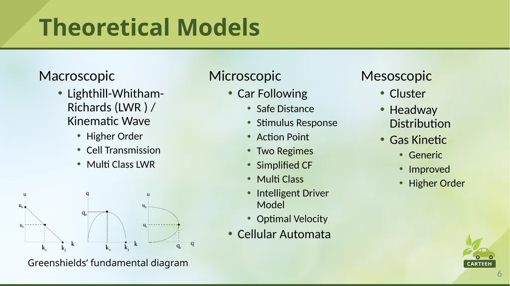
slide6. Theoretical Models Macroscopic
Lighthill-Whitham-Richards (LWR ) / Kinematic Wave
Higher Order
Cell Transmission
Multi Class LWR Microscopic
Car Following
Safe Distance
Stimulus Response
Action Point
Two Regimes
Simplified CF
Multi Class
Intelligent Driver Model
Optimal Velocity
Cellular Automata Mesoscopic
Cluster
Headway Distribution
Gas Kinetic
Generic
Improved
Higher Order Greenshields’ fundamental diagram<br>
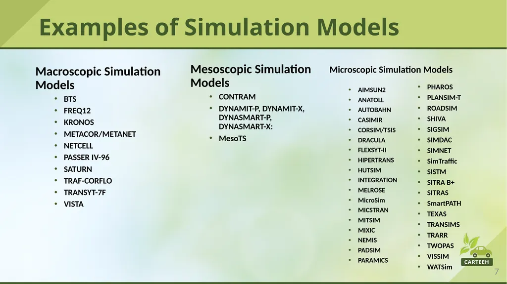
slide7. Examples of Simulation Models Macroscopic Simulation Models
BTS
FREQ12
KRONOS
METACOR/METANET
NETCELL
PASSER IV-96
SATURN
TRAF-CORFLO
TRANSYT-7F
VISTA Mesoscopic Simulation Models
CONTRAM
DYNAMIT-P, DYNAMIT-X, DYNASMART-P, DYNASMART-X:
MesoTS Microscopic Simulation Models

AIMSUN2
ANATOLL
AUTOBAHN
CASIMIR
CORSIM/TSIS
DRACULA
FLEXSYT-II
HIPERTRANS
HUTSIM
INTEGRATION
MELROSE
MicroSim
MICSTRAN
MITSIM
MIXIC
NEMIS
PADSIM
PARAMICS PHAROS
PLANSIM-T
ROADSIM
SHIVA
SIGSIM
SIMDAC
SIMNET
SimTraffic
SISTM
SITRA B+
SITRAS
SmartPATH
TEXAS
TRANSIMS
TRARR
TWOPAS
VISSIM
WATSim<br>
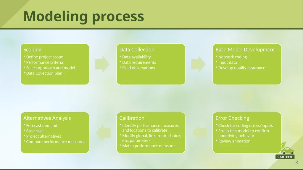
slide8. Modeling process<br>
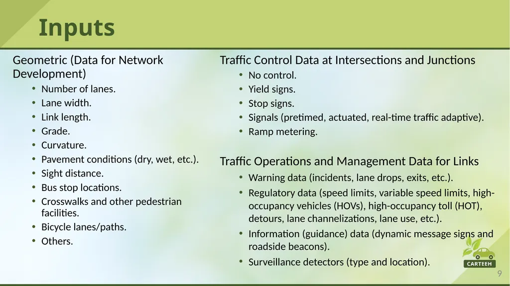
slide9. Inputs Geometric (Data for Network Development)
Number of lanes.
Lane width.
Link length.
Grade.
Curvature.
Pavement conditions (dry, wet, etc.).
Sight distance.
Bus stop locations.
Crosswalks and other pedestrian facilities.
Bicycle lanes/paths.
Others. Traffic Control Data at Intersections and Junctions
No control.
Yield signs.
Stop signs.
Signals (pretimed, actuated, real-time traffic adaptive).
Ramp metering. Traffic Operations and Management Data for Links
Warning data (incidents, lane drops, exits, etc.).
Regulatory data (speed limits, variable speed limits, high-occupancy vehicles (HOVs), high-occupancy toll (HOT), detours, lane channelizations, lane use, etc.).
Information (guidance) data (dynamic message signs and roadside beacons).
Surveillance detectors (type and location).<br>
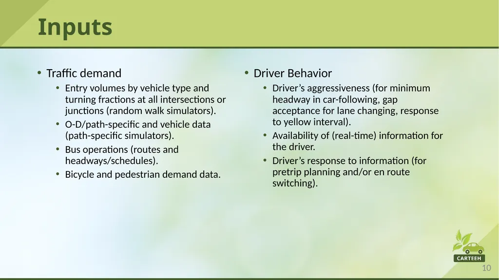
slide10. Inputs Traffic demand
Entry volumes by vehicle type and turning fractions at all intersections or junctions (random walk simulators).
O-D/path-specific and vehicle data (path-specific simulators).
Bus operations (routes and headways/schedules).
Bicycle and pedestrian demand data. Driver Behavior
Driver’s aggressiveness (for minimum headway in car-following, gap acceptance for lane changing, response to yellow interval).
Availability of (real-time) information for the driver.
Driver’s response to information (for pretrip planning and/or en route switching).<br>
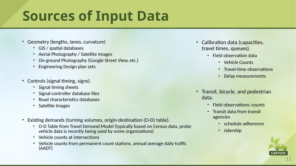
slide11. Sources of Input Data Geometry (lengths, lanes, curvature)
GIS / spatial databases
Aerial Photography / Satellite Images
On-ground Photography (Google Street View, etc.)
Engineering Design plan sets

Controls (signal timing, signs).
Signal timing sheets
Signal controller database files
Road characteristics databases
Satellite Images

Existing demands (turning volumes, origin-destination (O-D) table).
O-D Table from Travel Demand Model (typically based on Census data, probe vehicle data is recently being used by some organizations)
Vehicle counts at intersections
Vehicle counts from permanent count stations, annual average daily traffic (AADT) Calibration data (capacities, travel times, queues).
Field observation data
Vehicle Counts
Travel-time observations
Delay measurements

Transit, bicycle, and pedestrian data.
Field observations: counts
Transit data from transit agencies
schedule adherence
ridership<br>
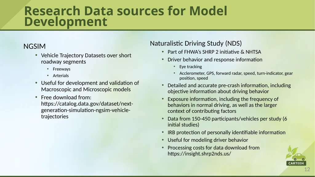
slide12. Research Data sources for Model Development NGSIM
Vehicle Trajectory Datasets over short roadway segments
Freeways
Arterials
Useful for development and validation of Macroscopic and Microscopic models
Free download from: https://catalog.data.gov/dataset/next-generation-simulation-ngsim-vehicle-trajectories Naturalistic Driving Study (NDS)
Part of FHWA’s SHRP 2 initiative & NHTSA
Driver behavior and response information
Eye tracking
Acclerometer, GPS, forward radar, speed, turn-indicator, gear position, speed
Detailed and accurate pre-crash information, including objective information about driving behavior
Exposure information, including the frequency of behaviors in normal driving, as well as the larger context of contributing factors
Data from 150-450 participants/vehicles per study (6 initial studies)
IRB protection of personally identifiable information
Useful for modeling driver behavior
Processing costs for data download from https://insight.shrp2nds.us/<br>
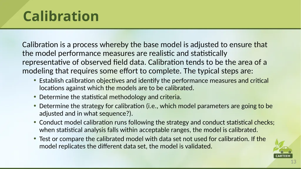
slide13. Calibration Calibration is a process whereby the base model is adjusted to ensure that the model performance measures are realistic and statistically representative of observed field data. Calibration tends to be the area of a modeling that requires some effort to complete. The typical steps are:
Establish calibration objectives and identify the performance measures and critical locations against which the models are to be calibrated.
Determine the statistical methodology and criteria.
Determine the strategy for calibration (i.e., which model parameters are going to be adjusted and in what sequence?).
Conduct model calibration runs following the strategy and conduct statistical checks; when statistical analysis falls within acceptable ranges, the model is calibrated.
Test or compare the calibrated model with data set not used for calibration. If the model replicates the different data set, the model is validated.<br>
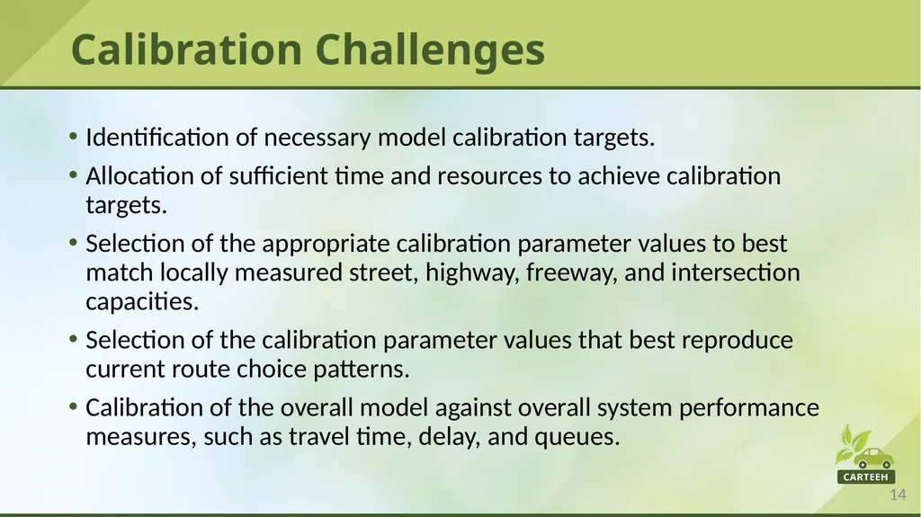
slide14. Calibration Challenges Identification of necessary model calibration targets.
Allocation of sufficient time and resources to achieve calibration targets.
Selection of the appropriate calibration parameter values to best match locally measured street, highway, freeway, and intersection capacities.
Selection of the calibration parameter values that best reproduce current route choice patterns.
Calibration of the overall model against overall system performance measures, such as travel time, delay, and queues.<br>
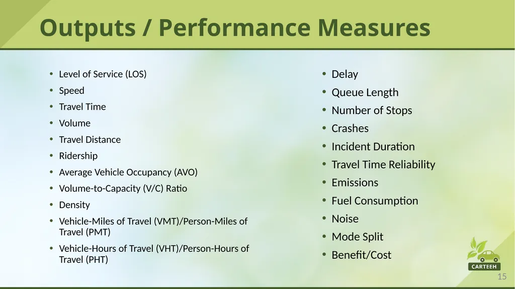
slide15. Outputs / Performance Measures Level of Service (LOS)
Speed
Travel Time
Volume
Travel Distance
Ridership
Average Vehicle Occupancy (AVO)
Volume-to-Capacity (V/C) Ratio
Density
Vehicle-Miles of Travel (VMT)/Person-Miles of Travel (PMT)
Vehicle-Hours of Travel (VHT)/Person-Hours of Travel (PHT) Delay
Queue Length
Number of Stops
Crashes
Incident Duration
Travel Time Reliability
Emissions
Fuel Consumption
Noise
Mode Split
Benefit/Cost<br>
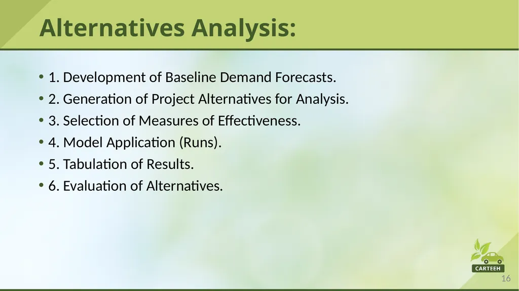
slide16. Alternatives Analysis: 1. Development of Baseline Demand Forecasts.
2. Generation of Project Alternatives for Analysis.
3. Selection of Measures of Effectiveness.
4. Model Application (Runs).
5. Tabulation of Results.
6. Evaluation of Alternatives.<br>
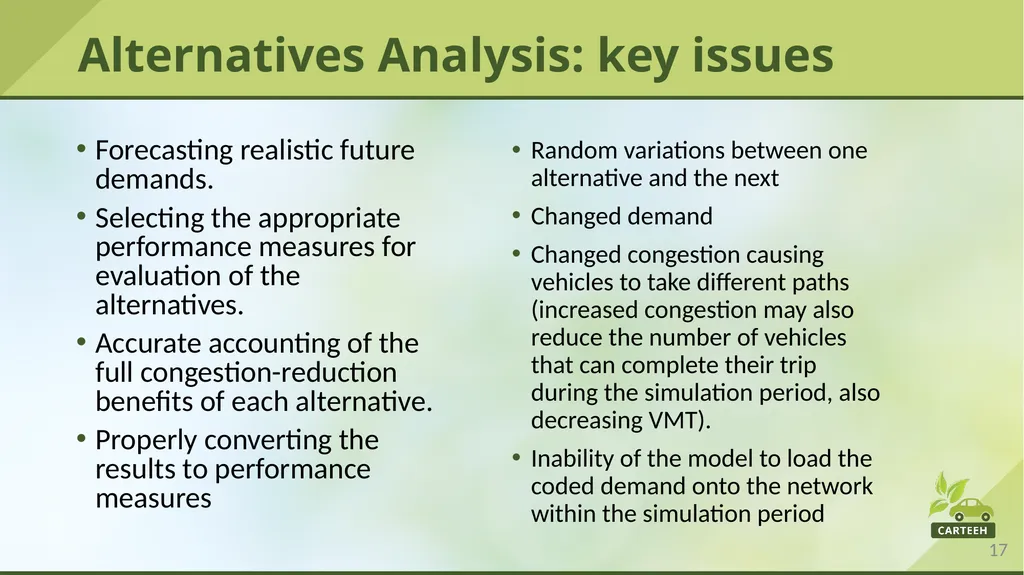
slide17. Alternatives Analysis: key issues Forecasting realistic future demands.
Selecting the appropriate performance measures for evaluation of the alternatives.
Accurate accounting of the full congestion-reduction benefits of each alternative.
Properly converting the results to performance measures Random variations between one alternative and the next
Changed demand
Changed congestion causing vehicles to take different paths (increased congestion may also reduce the number of vehicles that can complete their trip during the simulation period, also decreasing VMT).
Inability of the model to load the coded demand onto the network within the simulation period<br>
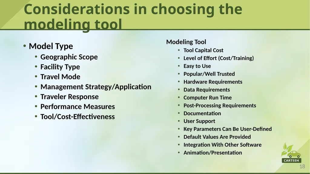
slide18. Considerations in choosing the modeling tool Model Type
Geographic Scope
Facility Type
Travel Mode
Management Strategy/Application
Traveler Response
Performance Measures
Tool/Cost-Effectiveness Modeling Tool
Tool Capital Cost
Level of Effort (Cost/Training)
Easy to Use
Popular/Well Trusted
Hardware Requirements
Data Requirements
Computer Run Time
Post-Processing Requirements
Documentation
User Support
Key Parameters Can Be User-Defined
Default Values Are Provided
Integration With Other Software
Animation/Presentation<br>
slide19. Discussion: Challenges and Limitations of using Modeling Availability of quality data
Limited empirical data
Data input and the diversity and inconsistency of data
Lack of understanding of the limitations of analytical tools
Tools may not be designed to evaluate all types of impacts produced by transportation strategies/applications
Desire to run real-time solutions.
Tendency to use simpler analytical tools and those available in house, although they might not be the best tools for the job
Biases against models and traffic analysis tools
Long computer run times<br>
slide20. Traffic Models help us understand traffic behavior, the capacities of road networks in serving demand, characteristics of demand and their relationship to changes in operational characteristics
Analytical models and traffic simulation helps us make data driven decisions and planning, incorporate future projections into the decision-making process and Evaluate/prioritize planning/operational alternatives before field implementation Discussion<br>
slide21. Flexibility of models to capture emerging scenarios (such as connected and autonomous vehicles or electric vehicles)
Calibration challenges of models
Ability of the theoretical models to capture transition between traffic flow states/regimes
Scalability of simulation models (run times)
Real-time / hybrid simulation Research Gaps and Future Directions<br>
slide22. Traffic modeling and simulation are resource and data intensive processes
Accurate scoping of the effort, commensurate with the goals and objectives of the decision making process are critical to the success
A wide variety of choices are available for modeling tools. Choice of modeling tools need to take into account the scope, resource availability, skillsets of human resources, etc. Take-Home Messages<br>
slide23. Extras<br>
slide24. Traveler Response Route Diversions: Captures changes in travel routes, including pre-trip route diversion and en route diversion.
Mode Shifts: Captures changes regarding the selection of travel modes.
Departure Time Choices: Captures changes in the time of travel.
Destination Changes: Represents changes to travel destinations.
Induced/Foregone Demand: Estimates new trips (induced demand) or foregone trips resulting from the implementation of traffic management strategies.<br>
slide25. Error checks Network Connectivity
Link Speed Limits
Intersection Geometry
Traffic Control<br>
slide26. Calibration / Validation Meaning of terms
Difference between terms/steps<br>
slide27. Use in Policy Decision Making Addressed in Introduction<br>
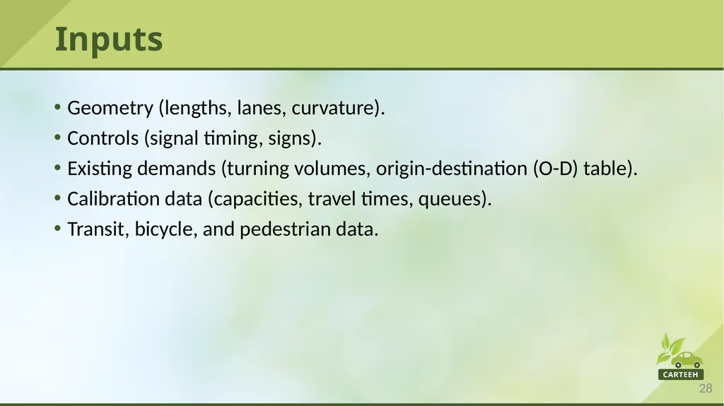
slide28. Inputs Geometry (lengths, lanes, curvature).
Controls (signal timing, signs).
Existing demands (turning volumes, origin-destination (O-D) table).
Calibration data (capacities, travel times, queues).
Transit, bicycle, and pedestrian data.<br>
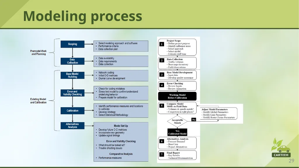
slide29. Modeling process<br>