/
1 Monte-Carlo Planning: Policy Improvement 1 Monte-Carlo Planning: Policy Improvement

1 Monte-Carlo Planning: Policy Improvement - PowerPoint Presentation

aaron
aaron . @aaron
Follow
342 views
Uploaded On 2019-06-22

1 Monte-Carlo Planning: Policy Improvement - PPT Presentation

Alan Fern 2 MonteCarlo Planning Often a simulator of a planning domain is available or can be learned from data 2 Fire amp Emergency Response Conservation Planning 3 Large Worlds MonteCarlo Approach ID: 759967

Share:

Link:

Embed:

Download Presentation from below link

Download Presentation The PPT/PDF document "1 Monte-Carlo Planning: Policy Improveme..." is the property of its rightful owner. Permission is granted to download and print the materials on this web site for personal, non-commercial use only, and to display it on your personal computer provided you do not modify the materials and that you retain all copyright notices contained in the materials. By downloading content from our website, you accept the terms of this agreement.


Presentation Transcript

Slide1

1

Monte-Carlo Planning:Policy Improvement

Alan Fern

Slide2

2

Monte-Carlo Planning

Often a simulator of a planning domain is availableor can be learned from data

2

Fire & Emergency Response

Conservation Planning

Slide3

3

Large Worlds: Monte-Carlo Approach

Often a simulator of a planning domain is availableor can be learned from dataMonte-Carlo Planning: compute a good policy for an MDP by interacting with an MDP simulator

3

World

Simulator

Real

World

action

State + reward

Slide4

4

MDP: Simulation-Based Representation

A

simulation-based representation

gives: S, A,

R

,

T

,

I

:

finite state set S (|S|=n and is generally very large)

finite action set A (|A|=m and will assume is of reasonable size)

Stochastic, real-valued, bounded reward function R(

s,a

) = r

Stochastically returns a reward

r

given input s and a

Stochastic transition function T(

s,a

) = s’ (i.e. a simulator)

Stochastically returns a state

s’

given input s and a

Probability of returning

s’

is dictated by

Pr

(s’ |

s,a

) of MDP

Stochastic initial state function I.

Stochastically returns a state according to an initial state distribution

These stochastic functions can be implemented in any language!

Slide5

5

Outline

You already learned how to evaluate a policy given a simulator

Just run the policy multiple times for a finite horizon and average the rewards

In next two lectures we’ll learn how to select good actions

Slide6

6

Monte-Carlo Planning Outline

Single State Case (multi-armed bandits)A basic tool for other algorithmsMonte-Carlo Policy ImprovementPolicy rolloutPolicy SwitchingMonte-Carlo Tree SearchSparse SamplingUCT and variants

Today

Slide7

7

Single State Monte-Carlo Planning

Suppose MDP has a single state and k actionsCan sample rewards of actions using calls to simulatorSampling action a is like pulling slot machine arm with random payoff function R(s,a)

s

a

1

a

2

a

k

R(s,a

1)

R(s,a2)

R(s,ak)

Multi-Armed Bandit Problem

Slide8

Multi-Armed Bandits

We will use bandit algorithms as components for multi-

state

Monte-Carlo planning

But they are useful in their own right

Pure

bandit problems arise in many applications

Applicable whenever:

We have a set of independent options with unknown utilities

There is a cost for sampling options or a limit on total samples

Want to find the best option or maximize utility of our samples

Slide9

Multi-Armed Bandits: Examples

Clinical Trials

Arms =

p

ossible treatments

Arm Pulls = application of treatment to

inidividual

Rewards = outcome of

treatment

Objective = Find best treatment quickly (debatable)

Online

Advertising

Arms = different ads/ad-types for a web page

Arm Pulls = displaying an ad upon a page access

Rewards = click through

Objective =

find

best add

quickly (the maximize clicks)

Slide10

10

Simple Regret Objective

Different applications suggest different types of bandit objectives.Today minimizing simple regret will be the objectiveSimple Regret Minimization (informal): quickly identify arm with close to optimal expected reward

s

a

1

a

2

a

k

R(s,a

1)

R(s,a2)

R(s,ak)

Multi-Armed Bandit Problem

Slide11

11

Simple Regret Objective: Formal Definition

Protocol: at time step n based on all prior observationsPick an “exploration” arm , then pull it and observe reward Pick an “exploitation” arm index that currently looks best (if algorithm is stopped at time it returns ) ( are random variables). Let be the expected reward of truly best armExpected Simple Regret (: difference between and expected reward of arm selected by our strategy at time n


Slide12

12

UniformBandit

Algorith (or Round Robin)

UniformBandit Algorithm: At round n pull arm with index (k mod n) + 1 At round n return arm (if asked) with largest average rewardI.e. is the index of arm with best average so farThis bound is exponentially decreasing in n! So even this simple algorithm has a provably small simple regret.


Theorem: The expected simple regret of Uniform after n arm pulls is upper bounded by O for a constant c.


Bubeck

, S.,

Munos

, R., &

Stoltz

, G. (2011). Pure exploration in finitely-armed and continuous-armed bandits. Theoretical Computer Science, 412(19), 1832-1852

Slide13

13

Can we do better?

Algorithm

-GreedyBandit : (parameter )At round n, with probability pull arm with best average reward so far, otherwise pull one of the other arms at random. At round n return arm (if asked) with largest average reward


Theorem: The expected simple regret of -Greedy for after n arm pulls is upper bounded by O for a constant c that is larger than the constant for Uniform(this holds for “large enough” n).


Tolpin, D. & Shimony, S, E. (2012). MCTS Based on Simple Regret. AAAI Conference on Artificial Intelligence.

Often is more effective than

UniformBandit

in practice.

Slide14

14

Monte-Carlo Planning Outline

Single State Case (multi-armed bandits)A basic tool for other algorithmsMonte-Carlo Policy ImprovementPolicy rolloutPolicy SwitchingMonte-Carlo Tree SearchSparse SamplingUCT and variants

Today

Slide15

Policy Improvement via Monte-Carlo

Now consider a very large multi-state MDP.Suppose we have a simulator and a non-optimal policy E.g. policy could be a standard heuristic or based on intuitionCan we somehow compute an improved policy?

15

World

Simulator+ Base Policy

Real

World

action

State + reward

Slide16

16

Policy Improvement Theorem

Definition: The Q-value function gives the expected future reward of starting in state s, taking action , and then following policy until the horizon h.How good is it to execute after taking action in state Define: Theorem [Howard, 1960]: For any non-optimal policy the policy is strictly better than . So if we can compute at any state we encounter, then we can execute an improved policyCan we use bandit algorithms to compute


Slide17

17

Policy Improvement via Bandits

s

a

1

a

2

a

k

SimQ

(s,a1,π,h)

SimQ(s,a2,π,h)

SimQ(s,ak,π,h)

Idea:

define a stochastic function

SimQ

(s,a,π,h) that we can implement and whose expected value is Qπ(s,a,h)Then use Bandit algorithm to select (approximately) the action with best Q-value (i.e. the action )


How to implement

SimQ

?

Slide18

18

Policy Improvement via Bandits

SimQ(s,a,π,h) q = R(s,a) simulate a in s s = T(s,a) for i = 1 to h-1 q = q + R(s, π(s)) simulate h-1 steps s = T(s, π(s)) of policy Return q

s

a1

a2

Trajectory under

p

Sum of rewards = SimQ(s,

a

1

,

π

,

h)

a

k

Sum of rewards = SimQ(s,

a

2

,

π

,

h)

Sum of rewards = SimQ(s,

a

k

,

π

,

h)

Slide19

19

Policy Improvement via Bandits

SimQ(s,a,π,h) q = R(s,a) simulate a in s s = T(s,a) for i = 1 to h-1 q = q + R(s, π(s)) simulate h-1 steps s = T(s, π(s)) of policy Return qSimply simulate taking a in s and following policy for h-1 steps, returning discounted sum of rewardsExpected value of SimQ(s,a,π,h) is Qπ(s,a,h)So averaging across multiple runs of SimQ quickly converges to Qπ(s,a,h)

Slide20

20

Policy Improvement via Bandits

s

a

1

a

2

a

k

SimQ

(s,a1,π,h)

SimQ(s,a2,π,h)

SimQ(s,ak,π,h)

Now apply your favorite bandit algorithm for simple regret

UniformRollout

: use

UniformBandit Parameters: number of trials n and horizon/height h-GreedyRollout : use -GreedyBandit Parameters: number of trials n, and horizon/height h( often is a good choice)


Slide21

21

UniformRollout

s

a

1

a

2

a

k

q

11

q

12

… q1w

q21 q22 … q2w

qk1 qk2 … qkw

SimQ(s,a

i

,

π

,

h) trajectories

Each simulates taking

action a

i

then following

π

for h-1 steps.

Samples of SimQ(s,a

i

,

π

,

h)

Each action is tried roughly the same number of times (approximately

times)


Slide22

22


s

a

1

a

2

a

k

q

11

q

12

q1u

q21 q22 … q2v

qk1

For

we might

expect it to be better than

UniformRollout

for

same value of n

.


Allocates a non-uniform number of trials across actions (focuses on more promising actions)

Slide23

23

Executing Rollout in Real World

s

a

1

a

2

a

k

a

1

a

2

a

k

a

2

a

k

run policy rollout

run policy rollout

Real world

state/action

sequence

Simulated

experience

How much time does each decision take?

Slide24

24

Policy Rollout: # of Simulator Calls

Total of n SimQ calls each using h calls to simulator and policy Total of hn calls to the simulator and to the policy (dominates time to make decision)

a

1

a

2

a

k

SimQ(s,a

i

,

π

,

h) trajectories

Each simulates taking

action a

i

then following

π

for h-1 steps.

s

Slide25

25

Practical Issues: Accuracy

Selecting number of trajectories n should be at least as large as the number of available actions(so each is tried at least once)In general n needs to be larger as the randomness of the simulator increases (so each action gets tried a sufficient number of times)Rule-of-Thumb : start with n set so that each action can be tried approximately 5 times and then see impact of decreasing/increasing nSelecting height/horizon h of trajectoriesA common option is to just select h to be the same as the horizon of the problem being solved Suggestion: setting h = -1 in our framework, which will run all trajectories until the simulator hits a terminal stateUsing a smaller value of h can sometimes be effective if enough reward is accumulated to give a good estimate of Q-values


In general, larger values are better, but this increases time.

Slide26

26

Practical Issues: Speed

There are three ways to speedup decision making time

Use a faster policy

Slide27

27

Practical Issues: Speed

There are three ways to speedup decision making time

Use a faster policy

Decrease the number of trajectories n

Decreasing Trajectories:

If n is small compared to # of actions k, then performance could be poor since actions don’t get tried very often

One way to get away with a smaller n is to use an

action filter

Action Filter:

a function f(s) that returns a subset of the actions in state s that rollout should consider

You can use your domain knowledge to filter out obviously bad actions

Rollout decides among the remaining actions returned by f(s)

Since rollout only tries actions in f(s) can use a smaller value of n

Slide28

28

Practical Issues: Speed

There are three ways to speedup either rollout procedure

Use a faster policy

Decrease the number of trajectories n

Decrease the horizon h

Decrease Horizon h:

If h is too small compared to the “real horizon” of the problem, then the Q-estimates may not be accurate

Can get away with a smaller h by using a

value estimation heuristic

Heuristic function:

a heuristic function v(s) returns an estimate of the value of state s

SimQ

is adjusted to run policy for h steps ending in state s’ and returns the sum of rewards up until s’ added to the estimate v(s’)

Slide29

29

Multi-Stage Rollout

A single call to Rollout[

π

,

h,w](s) yields one iteration of policy improvement starting at policy

π

We can use more computation time to yield multiple iterations of policy improvement via nesting calls to Rollout

Rollout[

Rollout[

π

,h,w]

,

h,w](s) returns the action for state s resulting from two iterations of policy improvement

Can nest this arbitrarily

Gives a way to use more time in order to improve performance

Slide30

30

Multi-Stage Rollout

a

1

a

2

a

k

Trajectories of

SimQ(s,a

i

,

Rollout[

π

,h,w]

,

h)

Each step requires

nh

simulator calls

for Rollout policy

Two stage: compute rollout policy of “rollout policy of

π

Requires

(

nh

)

2

calls to the simulator for 2 stages

In general exponential in the number of stages

s

Slide31

31

Example: Rollout for Solitaire [Yan et al. NIPS’04]

Multiple levels of rollout can payoff but is expensive

Player

Success Rate

Time/Game

Human Expert

36.6%

20 min

(naïve) Base Policy

13.05%

0.021 sec

1 rollout

31.20%

0.67 sec

2 rollout

47.6%

7.13 sec

3 rollout

56.83%

1.5 min

4 rollout

60.51%

18 min

5 rollout

70.20%

1 hour 45 min

Slide32

32

Rollout in 2-Player Games

s

a

1

a

2

a

k

q

11

q

12

… q1w

q21 q22 … q2w

qk1 qk2 … qkw

SimQ simply uses the base policy

to select moves for both players until the horizon

Rollout is biased toward

playing well against

Is this ok?


p1

p2

Slide33

33

Another Useful Technique: Policy Switching

Suppose

you have a set of base policies {

π

1

,

π

2

,…,

π

M

}

Also suppose that the best policy to use can depend on the specific state of the system and we don’t know how to

select.

Policy switching is a simple way to select which policy to use at a given step via a simulator

Slide34

34

Another Useful Technique: Policy Switching

s

Sim

(s,

π

1

,h)

Sim(s,π2,h)

Sim(s,πM,h)

The stochastic function

Sim

(s,

π,h) simply samples the h-horizon value of π starting in state sImplement by simply simulating π starting in s for h steps and returning discounted total rewardUse Bandit algorithm to select best policy and then select action chosen by that policy

π 1

π 2

π

M

Slide35

35

PolicySwitching

PolicySwitch[{π1, π2,…, πM},h,n](s) Define bandit with M arms giving rewards Sim(s,πi,h) Let i* be index of the arm/policy selected by your favorite bandit algorithm using n trialsReturn action πi*(s)

s

π

1

π

2

π

M

v

11

v

12

… v1w

v21 v22 … v2w

vM1 vM2 … vMw

Sim

(s,

π

i

,

h

) trajectories

Each simulates

following

π

i

for h steps.

Discounted cumulative

rewards

Slide36

36

Executing Policy Switching in Real World

s

1


𝜋

2

𝜋

k

𝜋

1

𝜋

2

𝜋

k

𝜋

2

(s)

𝜋

k

(s’)

run policy rollout

run policy rollout

Real world

state/action

sequence

Simulated

experience

Slide37

37

Policy Switching: Quality

Let denote the ideal switching policy Always pick the best policy index at any state The value of the switching policy is at least as good as the best single policy in the setIt will often perform better than any single policy in set.For non-ideal case, were bandit algorithm only picks approximately the best arm we can add an error term to the bound.


Theorem: For any state s, .


Slide38

Policy Switching in 2-Player Games

Suppose we have a two sets of polices, one for each player. Max Policies (us) : Min Policies (them) : }These policy sets will often be the same, when players have the same actions sets. Policies encode our knowledge of what the possible effective strategies might be in the gameBut we might not know exactly when each strategy will be mosteffective.


Slide39

Minimax Policy Switching

….….….….….….….….….

Build GameMatrix


Game Simulator

Current

State s

Each entry gives estimated value (for max player)

of playing a policy pair against one another

Each value estimated by averaging across

w simulated games

.

Slide40

MaxiMin Switching

….….….….….….….….….

Build GameMatrix


Game Simulator

Current

State s

MaxiMin

Policy


Select action


Can switch between policies based on state of game!

Slide41

MaxiMin Switching

….….….….….….….….….

Build GameMatrix


Game Simulator

Current

State s

Parameters in Library Implementation:

Policy Sets:

, }Sampling Width w : number of simulations per policy pairHeight/Horizon h : horizon used for simulations