The Monte Carlo Simulation - PDF document

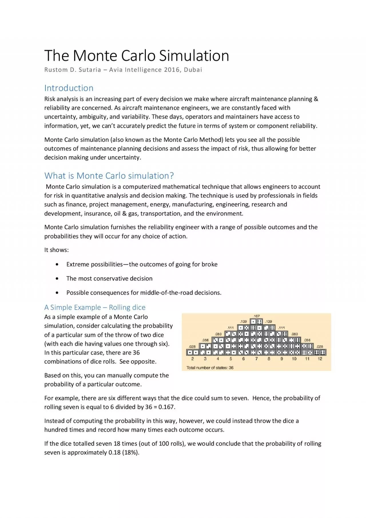
The Monte Carlo Simulation Rustom D. Sutaria – Avia Intelligence 2016 , Dubai Introduction Risk analysis is an increasing part of every decision we make where aircraft maintenance planning & reliability are concerned . As aircraft maintenance engineers, w e are constantly faced with uncertainty, ambiguity, and variability. These days, operators and maintainers have access to information, yet, we can’t accurately predict the future in terms of system or component reliability . Monte Carlo simulation (also kn own as the Monte Carlo Method) lets you see all the p ossible outcomes of maintenance planning decisions and assess the impact of risk, thus allowing for better decision making under uncertainty. What is Monte Carlo simulation? Monte Carlo simulation is a computerized mathemati cal technique that allows engineers to account for risk in quantitative analysis and decision making. The technique is used by profess ionals in fields such as finance, project management, energy, manufacturing, engineering, research a nd development, insurance, oil & gas, transportation, and the environment. Monte Carlo simulat ion furnishes the reliability engineer with a range of possible outcomes and the probabilities they will occur for any choice of action. It shows:  E xtreme possi bilities — the out comes of going for broke  T he most conse rvative decision  P ossible consequences for middle - of - the - road decisions. A Simple Example – Rolling dice As a simple example of a Monte Carlo simulation, consider calculating the probability of a part icular sum of the throw of two dice (with each die having values one through six). In this particular case, there ar e 36 combinations of dice rolls. See opposite. Based on this, you can manually compute the probability of a particular outcome. For examp le, th

ere are six different ways that the dice could sum to seven. Hence, the probability of rolling seven is equal to 6 divided by 36 = 0.167. Instead of computing the probability in this way, however, we could instead throw the dice a hundred times and record how many times each outcome occurs. If the dice totalled seven 18 times (out of 100 rolls), we would conclude that the probability of rolling seven is approximately 0.18 (18%). Obviously, the more times we rolled the dice, the less approximate ou r result would be. Better than rolling dice a hundred times, we can easily use a computer to simulate rolling the dice 10,000 times (or more). Because we know the probability of a particular outcome for one die (1 in 6 for all six numbers), this is simple. The output of 10,000 realiz ations could look like this: How Monte Carlo simulation works Monte Carlo simulation performs risk analysis by building models of possible results by substituting a range of values — a probability distribution — for any factor that has inherent uncertainty. It then calculates results over and over, each time using a dif ferent set of random values from the probability functions. Depending upon the number of uncertainties and the ranges specified for them, a Monte Carlo simulation could involve thousands or tens of thousands of recalculations before it is complete. Monte Carlo simulation produces distributions of possible outcome values. Using Probability Distributions By using probability distributions, variables can have different probabilities of different outcomes occurring. Probability distributions are a much more realistic way of describing uncertainty in variables of a risk analysis. Common probability distributions include: Normal – Or “bell curve.” The user simply defines the mean or expected value and a standard deviation to describe the

variation about the m ean. Values in the middle near the mean are most likely to occur. It is symmetric and describes many natural phenomena such as people’s heights. Examples of variables described by normal distributions include inflation rates and energy prices. Lognorma l – Values are positively skewed, not symmetric like a normal distribution. It is used to represent values that don’t go below zero but have unlimited positive potential. Examples of variables described by lognormal distributions include real estate prop erty values, stock prices, and oil reserves. Uniform – All values have an equal chance of occurring, and the user simply defines the minimum and maximum. Examples of variables that could be uniformly distributed include manufacturing costs or future sale s revenues for a new product. Triangular – The user defines the minimum, most likely, and maximum values. Values around the most likely are more likely to occur. Variables that could be described by a triangular distribution include past sales history pe r unit of time and inventory levels. PERT - The user defines the minimum, most likely, and maximum values, just like the triangular distribution. Values around the most likely are more likely to occur. However values between the most likely and extremes a re more likely to occur than the triangular; that is, the extremes are not as emphasized. An example of the use of a PERT distribution is to describe the duration of a task in a project management model. Discrete – The user defines specific values that ma y occur and the likelihood of each. An example might be the results of a lawsuit: 20% chance of positive verdict, 30% change of negative verdict, 40% chance of settlement, and 10% chance of mistrial. Method During a Monte Carlo simulation, values are sam pled at random from the input probabili

ty distributions. Each set of samples is called an iteration, and the resulting outcome from that sample is recorded. Monte Carlo simulation does this hundreds or thousands of times, and the result is a probabilit y distribution of possible outcomes. In this way, Monte Carlo simulation provides a much more comprehensive view of what may happen. It tells you not only what could happen, but how likely it is to happen. How Accurate are the Results? The accuracy of a Monte Carlo simulation is a function of the number of realizations. What we are talking about here refers to levels of confidence. The more iterations/realizations are computed the higher the confidence level. Which analysis would you trust? The Advantages of Monte Carlo Simulation  Probabilistic Results . Results show not only what could happen, but how likely each outcome is.  Graphical Results . Because of the data a Monte Carlo simulation generates, o it’s easy to create graphs of different outcomes and their chances of occurrence. o This is important for communicating findings to ot her stakeholders.  Sensitivity Analysis – Allows the analyst to easily to see which inputs had the biggest effect on bottom - line results.  Scenario Analys is - A nalysts can see exactly which inputs had which values together when certain outcomes occurred. Th is is invaluable for pursuing further analysis.  Correlation of Inputs . In Monte Carlo simulation, it’s possible to model interdependent relationships between input variables. It’s important for accuracy to represent how, in reality, when some factors goes up, others go up or down accordingly. Chance of rolling a 7 @18% after 1000 simulated roles & 95% confidence level Chance of rolling a 7 @25% after 100 simulated roles & 5% confidence lev