PPT-Post hoc tests

Author : alexa-scheidler | Published Date : 2017-05-23

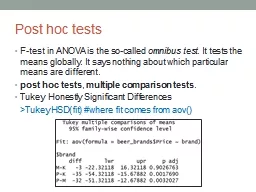
Ftest in ANOVA is the socalled omnibus test It tests the means globally It says nothing about which particular means are different post hoc tests multiple comparison

Presentation Embed Code

Download Presentation

Download Presentation The PPT/PDF document "Post hoc tests" is the property of its rightful owner. Permission is granted to download and print the materials on this website for personal, non-commercial use only, and to display it on your personal computer provided you do not modify the materials and that you retain all copyright notices contained in the materials. By downloading content from our website, you accept the terms of this agreement.

Post hoc tests: Transcript

Ftest in ANOVA is the socalled omnibus test It tests the means globally It says nothing about which particular means are different post hoc tests multiple comparison tests Tukey Honestly Significant . g shooter detection Goals of clock synchronization Compensate offset between clocks Compensate drift between clocks terms are explained on following slides Time Synchronization Sensing Localization Duty Cycling TDMA Ad Hoc and Sensor Networks Roger W MansionFirst is a Cambridge Objective First Certificate 1 15 This popular First Certificate course has been On the THE ANNUAL MSF METHODIST CONFERENCE LECTURE 2010 Given at Portsmouth by Revd Daniel Morris Chapma n peiverfissoclogse University o Cause & Effect. There are two important fallacies, where both assume that the timing of two variables relative to each other, in and of itself, is sufficient to establish that one is the cause and the other is the effect. This assumption is wrong.. Ad-hoc . On-Demand Distance Vector . Routing. &. DSR. : The Dynamic Source Routing . Protocol for. . Multi-Hop . Wireless Ad Hoc Networks. November 2011,. Giorgos . Papadakis. & Manolis. EETS 8316 wireless networks. . SUBMITTED BY. . ONKAR BIWALKAR SMU ID : 39603152. Fallacies. The ten deadly fallacies. Ad . Ignorantiam. Claiming something is true. because it cannot be proved to be false. Hasty generalization. Generalizing from insufficient evidence. Post hoc ergo propter hoc. Intro to Ad Hoc Networks. Announcements. Makeup lecture this Friday, 2/7, 12-1:15pm in Packard 312. Paper summary 1 due today. P. roposal feedback sent, . revision due . Monday 2/10. HW 1 . posted, . ad hoc meeting on DREGS. IETF-76. Mary Barnes (Dispatch WG co-chair). Eric Burger (ad hoc chair). 12 November 2009. 1. DREGS ad hoc (DISPATCH) IETF 76, Hiroshima, Japan. Remote Logistics. mp3 Feed: SPEAK INTO THE MICROPHONE!!!. Aimee Bernard. Greg Buck. Manuela Gardner. Erica Suchman. Jenny Taylor. Alan . Vajda. Facilitator: Tina Garza. Teachable Unit: Epigenetics. Tidbit: ‘Are you what your parents ate?’. The Tidbit within the . Danna Fabella, Statewide Linkages Coordinator. Peer Advisors. John Palm, Staff Services Analyst, Merced County. Rebecca . Wissing. , Administrative Analyst, Humboldt County. August 7, 2012. Agenda. Introductions:. Definition. relating to or being the fallacy of arguing from temporal sequence to a causal relation. Modern Example. . I ate a loaf of bread, and got a cold a few days later. Therefore, I must have gotten sick from the bread I ate. Cedar Mountain post acute rehabilitation center provide a therapeutic environment for our residents Yucaipa. Individualized treatment programs are developed with the interdisciplinary team of nursing, social services, Healthcare and dietary in consultation with your physicians. User. Presented by: Doug Greer | Prepared On: April 18, 2015. Overview. Navigating the Advanced Reporting Waters. Viewing Existing Reports. Creating an Ad-Hoc View. Understanding Domains. Ad-Hoc Views – In Depth. ork and What it Means to be an Engaged Commissioner on the . Economic Development Advisory Commission. Sharon Virts. January 9, 2015. Ad Hoc Committees. and EDAC Membership. What are Ad Hoc Committees.

Download Document

Here is the link to download the presentation.
"Post hoc tests"The content belongs to its owner. You may download and print it for personal use, without modification, and keep all copyright notices. By downloading, you agree to these terms.