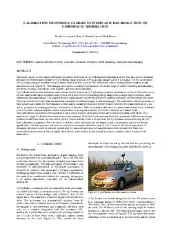
CALIBRATION OF FISHEYE CAMERA SYSTEMS AND THE REDUC TION OF CHROMATIC ABERRATION Frank - PDF document

CALIBRATION OF FISHEYE CAMERA SYSTEMS AND THE REDUCTION OF CHROMATIC ABERRATION Frank A. van den Heuvel, Ruud Verwaal, Bart Beers CycloMedia Technology B.V., P.O.box 68, NL - 4180 BB Waardenburg, E-mail: { FvandenHeuvel, RVerwaal, BBeers}@cyclomedia.nl Commission V, WG V/1 KEY WORDS: Camera calibration, fisheye, panorama, chromatic aberration, mobile mapping, omni-directional imaging ABSTRACT: This paper reports on the camera calibration procedure developed at CycloMedia and its modification for the reduction of chromatic Figure 1: CycloMedia car with camera system. and can be directly computed from its location in the image. Obtaining a panorama with this property from two partly overlapping fisheye images requires the camera – lens combination to be calibrated, i.e. the interior orientation is to be known. This calibration and its dependency on wavelength is the topic of this paper. Figure 2: Sample Cyclorama 1.2Previous work In the last years there is a growing interest in panoramic imaging and photogrammetric use of panoramic imagery. This is reflected in the success of ISPRS workshops on this topic. Several papers have been published on the calibration of panoramic camera systems that make use of a fisheye lens. Some approaches make use of straight line features (Amiri Parian and Grün, 2005), mostly a point field is used of which the 3D coordinates of the targets are known (Kannala and Brandt, 2004; Schneider and Schwalbe, 2005; Schwalbe, 2005). The calibration method presented here makes use of point features, however, spatial coordinates of the targets are not required. Recently, some investigations into the elimination of lateral chromatic aberration have been conducted (Kaufmann and Ladstädter, 2005; Luhmann, 2006; Schwalbe and Maas, 2006). These studies aim at image enhancement or photogrammetric measurement precision improvement. Only in (Schwalbe and Maas, 2006) chromatic aberration of a fisheye camera system is considered. In all approaches a calibration procedure is applied separately for each colour band instead of only one band, usually green. Thus, a set of calibration parameters is determined for each colour band. In this paper we apply the same approach using the calibration method developed in-house. 1.3Paper contentIn section 2 the camera model adopted by CycloMedia is presented as well as the camera calibration procedure developed in-house. The precision of the calibration is demonstrated with an example. In section 3 the nature of chromatic aberration is explained and how we use our calibration procedure for determining lateral chromatic aberration. An example shows its limited applicability and how a significant reduction is obtained with a manual approach. The paper finishes with conclusions in section 4. Website of the last workshop: http://www2.informatik.hu-berlin.de/sv/pr/PanoramicPhotogrammetryWorkshop2005/ 2.CAMERA CALIBRATION 2.1The camera model In (Kannala and Brandt, 2004) an overview of different camera models is given. The perspective projection of a pinhole camera is described with: q tan = (1) where r = distance image point – principal point = focal length = angle between optical axis and incoming ray Figure 3: Fisheye projection (schematic). For a fisheye lens the straightforward so-called f-theta mapping (Kumler and Bauer, 2000) is most common and used here. This projection is also called equiangular (Schwalbe and Maas, 2006) and equidistance projection (Kannala and Brandt, 2004): q × = (2) The parameters r and are depicted in Figure 3. The design of the fisheye lens used here is approaching this relation within a tolerance of ±6%, according to the specifications of the manufacturer. We model the deviations from the relation in (2) with a polynomial: 1( (3) The number of parameters to be estimated (the order of the polynomial) can be set by the user. Next to the parameters and in (3), the camera model is complete with the parameters (, ) representing the location of the principal point. For an image point with location (x, y), r is computed as follows: (4) To compute the spatial direction vector of a ray in space associated with an image point, an iterative procedure is applied based on equations (3) and (4) to find angle . The angle in the image plane found with: arctan( - (5) Equations (4) and (5) define the transformation from Cartesian to Polar co-ordinates in the image plane. The inverse of r lens optical axis equation (3) represents the step to a spatial direction in spherical co-ordinates (, ). 2.2The calibration procedureBefore the camera is calibrated the fisheye lens is mounted, focussed, and fixed in a specially designed frame in order to guarantee the long-term stability of the interior orientation. The procedure for the calibration of a fisheye camera consists of the following steps: 1.Acquisition of four images in a calibration room taken at 90º horizontal angles. The room contains 100 black circular targets on a white background, a sample image is shown in Figure 4. 2.Semi-automatic measurement of tie points (3D co-ordinates of these points are unknown) and establishment of correspondence. 3.Least-squares adjustment for camera parameter estimation. Apart from the camera parameters, a horizontal yaw angle is estimated for each image except one. Furthermore, a roll and a pitch parameter are estimated. The mathematical model consists of two observation equations per point measured: one for the horizontal and one for the vertical angle. Figure 4: Sample calibration image. 2.3Example The procedure above is regularly applied at CycloMedia for the calibration of the current 27 camera systems. Here we present an example in which the in-house developed sub-pixel image measurement has been compared with the target detection and sub-pixel measurement offered by the software package PhotoModeler (Eos Systems Inc, 2006). More than 90% of the targets were automatically detected by this software. The in-house developed software uses a centre of gravity approach as does the method offered by PhotoModeler. However, the latter is weighted. Here we name the first method “centroid” and the second “weighted centroid”. PhotoModeler’s least-squares template matching method (LSM) has also been tested. No significant differences in the results were found; the estimated standard deviation decreased only marginally from 0.16 to 0.15 pixel. The measurements of 4 fisheye images have been processed with the adjustment software developed by CycloMedia. The results of the least-squares parameter estimation are summarised in Table 1. Image Point Measurement Centroid Weighted Centroid estimated (pix) 0.16 0.16 Roll (deg) 0.046 (0.005) 0.049 Pitch (deg) -0.049 (0.027) -0.050 Yaw1 (deg) 181.028 (0.017) 181.022 Yaw2 (deg) 269.878 (0.017) 269.873 Yaw3 (deg) 90.673 (0.015) 90.673 (pix) 1736.55 (0.39) 1736.66 (pix) 1128.54 (0.71) 1128.41 (pix/rad) 763.89 (3.25) 762.35 0.0133 0.0243 -0.0596 -0.0815 0.0589 0.0754 -0.0240 -0.0283 Table 1: Comparison of adjustment results using different image measurement methods (standard deviation between brackets, identical for ‘weighted centroid’). Roll and pitch are the angles of the camera system relative to the rotation axis. The yaw of the first image is set to zero. Note that only the green colour band of the imagery has been used. In conclusion, no differences changes between the results of the two packages were observed. Changes in the focal length and the polynomial parameters are difficult to interpret due to the correlation between them; for angles with the optical axis smaller than 90º the difference in radius is below 1 pixel. 3.CHROMATIC ABERRATION 3.1What is chromatic aberration? Chromatic aberrations are imperfections in the imaging properties of a lens due to the dependency of the refractive index of the lens material on the wavelength of the light. The two main types of chromatic aberrations are longitudinal (or axial) chromatic and lateral (or oblique) aberration (Fiete, 2004) and (Kaufmann and Ladstädter, 2005). Figure 5: Longitudinal aberration Figure 6: Lateral aberration Longitudinal aberration results in a focal length that is wavelength dependent. In other words, it is not possible to focus all wavelengths at one position of the image plane (Figure 5). Lateral aberration results in a wavelength dependent radial displacement of an image point that, at least approximately, leads to a wavelength dependent image magnification (Figure 6). In this paper we concentrate on the latter type of aberration because it is the most prominent type in the imagery at hand. 3.2Determining lateral chromatic aberration As demonstrated in (Kaufmann and Ladstädter, 2005), (Schwalbe and Maas, 2005), and (Hastedt et al., 2006), lateral chromatic aberration can be determined by applying a standard camera calibration to each of the three colour bands. 50100150200250145147149151153155157159161163165 red green blue 5010015020025015202530354045 red green blue Figure 7: Sample target (small) located close to the right image border (Figure 4), top-left: original, top-middle: red minus green band (stretched), top-right: target in image centre, middle and bottom: RGB profile in column direction of a small and a large target. The use of a separate set of camera calibration parameters for each colour band in further processing allows the elimination of the visually apparent lateral aberration (Figure 7) and improves measurement precision. However, as shown in the example in the next section, this procedure was not successful for the imagery under consideration. 3.3Example Each colour band of four images with 90 degree horizontal angular separation have been measured with both the CycloMedia semi-automatic measurement tool and PhotoModeler’s automatic target detection. The measurement results of the 94 respectively 92 targets are shown in the figures below and the statistics in Table 2. 6007008009001000110012001300140050010001500200025003000 band0 band1 band2 Figure 8: Centroid point measurements; shift relative to green band1 is enlarged with a factor 100. 6007008009001000110012001300140050010001500200025003000 band0 band1 band2 Figure 9: Weighted centroid point measurement; shift relative to green band1 is enlarged with a factor 100. Colour bands Centroid x, y (pixel) Weighted Centroid x, y (pixel) Red - Green RMS 0.31, 0.15 0.23, 0.16 min. -0.51, -0.49 -0.52, -0.87 max. 0.64, 0.21 0.57, 0.15 (pix/rad) +0.30 +0.20 Blue - Green RMS 0.13, 0.10 0.53, 0.24 min. -0.32, -0.38 -1.08, -0.75 max. 0.24, 0.24 0.79, 0.93 f (pix/rad)+0.03 +0.52 Table 2: Differences between colour bands for the two measurement methods. In Table 2 the change in focal length is computed with the lens distortion parameters fixed. The values used were estimated using the green band. It clearly shows the image magnification of the red and blue bands relative to green; at an angle of 90 degree between optical axis and incoming ray the largest mean shift is 0.82 pixel (0.52/2) found with the weighted centroid method in the blue band. Six sets of camera parameters (one for each combination of three colours and two measurement methods) were estimated with CycloMedia’s adjustment software. The estimated standard deviation was close to 0.16 pixel for all adjustments. For each measurement method the RGB images were resampled to a spherical panorama, each with its own set of camera parameters. An example (based on the weighted centroid method) is shown in Figure 10. Figure 10: Part of a spherical panorama after merging three colour bands processed with colour specific calibration parameters. Comparison with a spherical panorama computed using a single set of calibration parameters based on the green band did not show any significant improvement. This is not surprising because the corrections applied are at the sub-pixel level, while the most visible colour aberration, i.e. the surplus of red in the black target (see Figure 7), spreads over 5 to 6 pixels in radial direction. This leads to the conclusion that for the visible colour aberration for the images under consideration, lateral chromatic aberration plays only a minor role. 3.4Manual reduction of chromatic aberration The question arises what causes the colour aberration apparent in Figure 7. No scientific literature on the subject could be found, however, on the Internet a type of colour aberration called “purple fringing” is discussed (Wikipedia, 2006). There is no agreement on the exact cause, but this colour aberration is frequently found in digital photography, especially with wide angle lenses, at large apertures, in the corners of the image (radial aberration), and in high contrast areas. Several image processing packages allow to manually correct for chromatic aberration. Commonly these packages allow to manually set a magnification for the red and blue colour band in order to improve the fit with the unaltered green band. We have tested Picture Window Pro 4.0. The results on the targets of Figure 7 are shown in Figure 11. 50100150200250140145150155160 red green blue 5010015020025010152025303540 red green blue Figure 11: Sample target (Figure 7), top-left: after manual correction of chromatic aberration, top-right: red minus green band (stretched), middle and bottom: RGB profile in column direction of a small and a large target. A significant visual improvement has been obtained. However, from Figure 11 it is clear that this does not fully correct the aberration. For a final solution more research into the nature of the problem is required. 4.CONCLUSIONS The paper presents the calibration procedure developed by CycloMedia for the processing of two overlapping fisheye images into a spherical panorama: a so-called Cyclorama. The least-squares adjustment involved in the calibration shows the semi-automatic target measurement to be accurate to the sub-pixel level with 0.16 pixel estimated standard deviation. This implies that the angular precision of well identifiable targets measured in a Cyclorama is 0.014º or better than 3 mm at 10 m. The calibration procedure has been applied for an estimation of a set of interior orientation parameters per colour band aiming at elimination of lateral chromatic aberration, firstly to improve the imagery visually, and secondly for improving the potential measurement precision. This approach was not successful because the corrections found were at the sub-pixel level while the visible chromatic aberration stretches over more than 5 pixels. With adjusting the magnification of the red and blue band manually it was possible to improve the visual appearance of the imagery significantly, however, more research is needed into the nature of the problem in order to develop a final solution. REFERENCES Amiri Parian, J. and Gruen, A., 2005. Panoramic Camera Calibration Using 3D Straight Lines. International Archives of Photogrammetry, Remote Sensing and Spatial Information Sciences, Vol. XXXVI, part 5/W8. ISPRS "Panoramic Photogrammetry Workshop", Berlin, Germany, 24-25 February 2005. Eos Systems Inc, 2006. Photogrammetric software package PhotoModeler version 5. http://www.photomodeler.com/pmpro01.html Accessed: July 2006. Fiete, R.D., 2004. Lens aberrations. In: Manual of Photogrammetry. Fifth edition, Section 4.1.6, J.Chris Mc Glone (ed.), American Society of Photogrammetry and Remote Sensing (ASPRS), ISBN 1-57083-071-1, pp. 346-349. Hastedt, H. Luhmann, T., Tecklenburg, W., 2006. Nutzung von RGB-Farbkanälen für die hochgenaue 3D-Punktmessung. Luhmann/Müller (ed.): Photogrammetrie, Laserscanning, Optische 3D-Messtechnik – Beiträge der 5. Oldenburger 3D-Tage, Wichmann Verlag, Heidelberg. Kannala, J. and Brandt, S., 2004. A generic camera calibration method for fish-eye lenses. In: proceedings 17th International Conference on Pattern Recognition (ICPR 2004), pp 10-13. Kaufmann, V. and Ladstädter, R., 2005. Elimination of color fringes in digital photographs caused by lateral chromatic aberration. Proceedings of the XX International Symposium CIPA 2005, 26 September - 1 October 2005, Turin, Italy, Vol. 1, 403-408 Kumler, J.J., Bauer, M., 2000. Fisheye lens designs and their relative performance. In: Proceedings of the Lens and Optical System Design and Engineering Conference of the SPIE Annual Meeting. Luhmann, Th., 2006. High precision photogrammetry using RGB colour information. In: proceedings ‘Coordinate Metrology Systems Conference CMSC2006’, July 2006. Schneider, D., Schwalbe, E., 2005. Design and testing of mathematical models for a full-spherical camera on the basis of a rotating linear array sensor and a fisheye lens. In: proceedings of ‘Optical 3D Measurement Techniques VII’, Eds.: Grün, A.; Kahmen, H., Vol.1, pp.245-254. Schwalbe, E, 2005. Geometric modelling and calibration of fisheye lens camera systems. Proceedings 2nd Panoramic Photogrammetry Workshop, Int. Archives of Photogrammetry and Remote Sensing, Vol. 36, Part 5/W8. Schwalbe, E., Maas, H-G., 2006. Ein Ansatz zur Elimination der chromatischen Abberation bei der Modellierung und Kalibrierung von Fisheye-Aufnahmesysteme. In Luhmann (ed.): Photogrammetrie – Laserscanning – Optische 3D-Messtechnik. Wichmann Verlag, Heidelberg. Wikipedia, 2006. Purple Fringing. http://en.wikipedia.org/wiki/Purple_fringing , Accessed: July 2006.