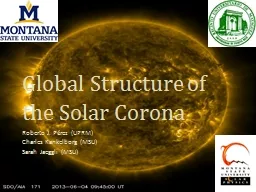
/
Global Structure of the Solar Corona Global Structure of the Solar Corona

Global Structure of the Solar Corona - PowerPoint Presentation

alida-meadow
alida-meadow . @alida-meadow
Follow
396 views
Uploaded On 2015-11-29

Global Structure of the Solar Corona - PPT Presentation

Roberto J Pérez UPRM Charles Kankelborg MSU Sarah Jaeggli MSU Abstract The AIA instrument on the Solar Dynamics Observatory obtains images of the sun in seven different extreme ultraviolet wavebands Each filter produces images with distinctive appearance that is apparent to exp ID: 209399

solar pixels contrast temperature pixels solar temperature contrast limb waveband 304 frequency angstroms wavebands characteristic arcsecs coronal bumps structures

Share:

Link:

Embed:

Download Presentation from below link

Download Presentation The PPT/PDF document "Global Structure of the Solar Corona" is the property of its rightful owner. Permission is granted to download and print the materials on this web site for personal, non-commercial use only, and to display it on your personal computer provided you do not modify the materials and that you retain all copyright notices contained in the materials. By downloading content from our website, you accept the terms of this agreement.


Presentation Transcript

Slide1

Global Structure of the Solar Corona

Roberto J. Pérez (UPRM)

Charles Kankelborg (MSU)Sarah Jaeggli (MSU)Slide2

Abstract

The AIA instrument on the Solar Dynamics Observatory obtains images of the sun in seven different extreme ultraviolet wavebands. Each filter produces images with distinctive appearance that is apparent to experienced observers. Subjective descriptions abound in the literature and in conference presentations, as do qualitative explanations of the physical reasons for these differences. We seek a quantitative description of the image properties, with the aim of understanding what the general image properties indicate about the temperature structure of the corona. Our preliminary results, obtained at multiple heliocentric angles above and below the limb, show that some channels consistently present a high or low intensity contrast which we attribute to the differing temperature, density and filling factor of the structures imaged. We also investigate the power spectra characteristic of each waveband. Slide3

Main Question

Why are images produced by different EUV (Extreme ultraviolet) filters so different? Can these differences be caused by physical parameters or could it be that different filters image specific solar structures?Slide4

Possible Explanations

Some papers present qualitative explanationsInstrument Scattering, Resonance Scattering and contamination of photons in the passbands has been suggested but they have been proven wrong

.“Filling-Factor Model” – Piling up of structures along the line of sightSlide5

Data

SDO (Solar Dynamics Observatory) (NASA) - AIA (Atmospheric Image Assembly)

We consider seven different EUV (Extreme Ultraviolet) wavebands.94 Angstroms131 Angstroms171 Angstroms193 Angstroms211 Angstroms304 Angstroms335 AngstromsSlide6

DataSlide7

Approach

Extract intensity arrays corresponding to different heliocentric annular regions.2^14 elements

Divide the arrays by their median value (For means of comparison)Compare these arrays using different techniques Slide8

Histograms

The histograms presented here were created by taking the average of histograms corresponding to twelve consecutive Carrington rotations of the sun (roughly).The frequency axis is log-scaledSlide9

200-205 pixelsSlide10

500-505 pixelsSlide11

1000-1005 pixelsSlide12

1500-1505 pixelsSlide13

1620-1625 pixelsSlide14

1700-1705 pixelsSlide15

1800-1805Slide16

Observations

High frequency of low intensity pixels in the 335 and 94 wavebandsRelatively similar structure among wavebandsSeemingly erratic

behavior far above the solar limb.Slide17

Contrast

We define contrast as the difference between the 75th percentile intensity value and the 25th percentile value.Slide18

200-205 pixelsSlide19

500-505 pixelsSlide20

1000-1005 pixelsSlide21

1500-1505 pixelsSlide22

1620-1625 pixelsSlide23

1700-1705 pixelsSlide24

1800-1805 pixelsSlide25

Observations

94, 335, and 211 consistently have the higher contrast in all annular regions. This does not support our initial hypothesis that the images that look less “fuzzier” to our eyes (ie

. 304) should have the higher contrast.The 304 waveband consistently presents a low contrast.The plots from annular regions below the limb look different from the ones above the limb. Imaging of different ionic species could be an explanation for this.Slide26

Contrast vs. Characteristic Temperature

It is possible to deduce a characteristic temperature for each waveband.This does not mean that everything imaged in that waveband is at that specific temperature but it provides a nice approximation.

Some ions are only imaged in specific solar activities (ie. Flares). For our purposes we use the most stable temperature that corresponds to each waveband.Slide27

200-205 pixelsSlide28

500-505 pixelsSlide29

1000-1005 pixelsSlide30

1500-1505 pixelsSlide31

1620-1625 pixelsSlide32

1700-1705 pixelsSlide33

Observations

For annular regions below the limb we can observe a light correlation between characteristic temperature and contrast.Annular regions above the solar limb show no correlation at all.

It is important to note that the waveband that has the lowest characteristic temperature almost always has the lowest contrast below the limb while the waveband that has the highest characteristic temperature almost always presents the highest contrast below the limb.304 is dominated by Si XI (Log(6.2)=6.2) above the limb.Slide34

Discrete Fourier Transforms

These plots consist of the average of Fourier transform plots corresponding to twelve consecutive Carrington rotations of the sun.The intensity component axis is log scaled The frequency axis is presented as log(frequency)

The frequency axis goes to the Nyquist frequencySlide35

200-205 pixelsSlide36

500-505 pixelsSlide37

1000-1005 pixelsSlide38

1500-1505 pixelsSlide39

1620-1625 pixelsSlide40

1700-1705 pixelsSlide41

1800-1805 pixelsSlide42

Observations

Linear behavior below the limbs (small bumps noticeable in the 94, 304 and 131 wavebands.Bumps become more noticeable above the limbs

Could the bumps be of solar origin?Mean Signal (335-94-131-304) : Bump height (94-335-131-304) (Highest to lowest)Period of some solar structures:Sunspots: ~33 arcsecsGranules: ~1.4-2.0 arcsecs (frequency range: (-1.7) – (-0.15))Supergranules

: ~49 arcsecsCoronal Holes: ~974-1252 arcsecsActive

Region Loops: ~14 arcsecsSpicules: ~.7 arcsecsSlide43

Overall Results

The characteristic temperature of a specific waveband seems to have an effect on the contrast observed. The temperature of the imaged structure of each waveband appears to directly affect the contrast or ‘fuzziness” that our eyes perceive.

It is possible that some temporary solar structures are affecting the overall consistency of the results (This needs further proof)The bumps on the Fourier transform plots seem to be of solar origin. Granular and supergranular scales look relevant.Hotter wavebands present bumps (Coronal heating problem?)Slide44

Further Work

Construction of a coronal model - Densities of the solar structures imaged - Temperature map of the plasma imaged by the different

wavebandsFind the origin of the bumps on the Fourier transform plots. Slide45

References

The Transparency of Solar Coronal Active Regions (Brickhouse & Shmelz, 2005)

Warm And Fuzzy: Temperature and Density Analysis of an Fe XV EUV Imaging Spectrometer Loop (Shmelz et al., 2011)Are Coronal Loops Isothermal or Multithermal? (Shmelz et al., 2009)SDO/AIA Response to Coronal Hole,

Quiet Sun, Active Region and Flare Plasma (O’Dwyer et al. , 2010)