1 W. Riegler/CERN Particle Detectors 1/2 - PowerPoint Presentation

ariel . @ariel

342 views
Uploaded On 2022-05-18

1 W. Riegler/CERN Particle Detectors 1/2 - PPT Presentation

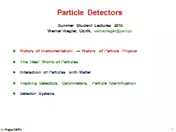
Werner Riegler CERN wernerrieglercernch 2 W RieglerCERN History of Particle Physics 1895 Xrays WC R ö ntgen 1896 Radioactivity H Becquerel 1899 Electron JJ Thomson ID: 911702

cern chamber cloud riegler chamber cern riegler cloud particle bubble rays geiger emulsion particles wilson counter cosmic nuclear wire

Link:

Copy

Embed:

<iframe width="560" height="315" src="https://www.docslides.com/embed/911702" frameborder="0" allowfullscreen></iframe>

Download Presentation from below link

Download Presentation The PPT/PDF document "1 W. Riegler/CERN Particle Detectors 1/2" is the property of its rightful owner. Permission is granted to download and print the materials on this web site for personal, non-commercial use only, and to display it on your personal computer provided you do not modify the materials and that you retain all copyright notices contained in the materials. By downloading content from our website, you accept the terms of this agreement.

Presentation Transcript

Slide1

W. Riegler/CERN

Particle Detectors 1/2

Werner

Riegler, CERN,

werner.riegler@cern.ch

Slide2

W. Riegler/CERN

History of Particle Physics

1895:

X-rays, W.C. R

ntgen

1896:

Radioactivity, H. Becquerel

1899:

Electron, J.J. Thomson

1911:

Atomic Nucleus, E. Rutherford

1919:

Atomic Transmutation, E. Rutherford

1920:

Isotopes, E.W. Aston

1920-1930:

Quantum Mechanics, Heisenberg, Schr

dinger, Dirac

1932:

Neutron, J. Chadwick

1932:

Positron, C.D. Anderson

1937:

Mesons, C.D. Anderson

1947:

Muon, Pion, C. Powell

1947:

Kaon, Rochester

1950:

QED, Feynman, Schwinger, Tomonaga

1955:

Antiproton, E. Segre

1956:

Neutrino, Rheines

etc. etc. etc.

Slide3

W. Riegler/CERN

History of Instrumentation

1906:

Geiger Counter, H. Geiger, E. Rutherford

1910:

Cloud Chamber, C.T.R. Wilson

1912:

Tip Counter, H. Geiger

1928:

Geiger-Müller Counter, W. M

ller

1929:

Coincidence Method, W. Bothe

1930:

Emulsion, M. Blau

1940-1950:

Scintillator, Photomultiplier

1952:

Bubble Chamber, D. Glaser

1962:

Spark Chamber

1968:

Multi Wire Proportional Chamber, C. Charpak

Etc. etc. etc.

Slide4

W. Riegler/CERN

On Tools and Instrumentation

“New directions in science are launched by new tools much more often than by new concepts.

The effect of a concept-driven revolution is to explain old things in new ways.

The effect of a tool-driven revolution is to discover new things that have to be explained”

From Freeman Dyson ‘Imagined Worlds’

Slide5

W. Riegler/CERN

History of Instrumentation

History of ‘Particle Detection’

Image Tradition:

Cloud Chamber

Emulsion

Bubble Chamber

Logic Tradition:

Scintillator

Geiger Counter

Tip Counter

Spark Counter

Electronics Image:

Wire Chambers

Silicon Detectors

…

Peter Galison, Image and Logic

A Material Culture of Microphysics

Slide6

W. Riegler/CERN

History of Instrumentation

Image Detectors

‘Logic (electronics) Detectors ’

Bubble chamber photograph

Early coincidence counting experiment

Slide7

W. Riegler/CERN

History of Instrumentation

Both traditions combine into the ‘Electronics Image’ during the 1970ies

Z-Event at UA1 / CERN

Slide8

W. Riegler/CERN

IMAGES

Slide9

W. Riegler/CERN

Cloud Chamber

John Aitken, *1839, Scotland:

Aitken was working on the meteorological question of

cloud formation. It became evident that cloud

droplets only form around condensation nuclei.

Aitken built the ‘Dust Chamber’ to do controlled

experiments on this topic. Saturated water vapor

is mixed with dust. Expansion of the volume leads to

super-saturation and condensation around the

dust particles, producing clouds.

From steam nozzles it was known and speculated that

also electricity has a connection to cloud formation.

Dust Chamber, Aitken 1888

Slide10

W. Riegler/CERN

Cloud Chamber

Charles Thomson Rees Wilson, * 1869, Scotland:

Wilson was a meteorologist who was, among other things, interested in cloud formation initiated by electricity.

In 1895 he arrived at the Cavendish Laboratory where J.J. Thompson, one of the chief proponents of the corpuscular nature of electricity, had studied the discharge of electricity through gases since 1886.

Wilson used a ‘dust free’ chamber filled with saturated water vapor to study the cloud formation

caused by ions present in the chamber.

Cloud Chamber, Wilson 1895

Slide11

W. Riegler/CERN

Cloud Chamber

Conrad R

öntgen discovered X-Rays in 1895.

At the Cavendish Lab Thompson and Rutherford found that irradiating a gas with X-rays increased it’s conductivity suggesting that X-rays produced ions in the gas.

Wilson used an X-Ray tube to irradiate his Chamber and found ‘a very great increase in the number of the drops’, confirming the hypothesis that ions are cloud formation nuclei.

Radioactivity (‘Uranium Rays’) discovered by Becquerel in 1896. It produced the same effect in the cloud chamber.

1899 J.J. Thompson claimed that cathode rays are

fundamental particles



electron.

Soon afterwards it was found that rays from radioactivity consist of alpha, beta and gamma rays (Rutherford).

This tube is a glass bulb with positive and negative electrodes, evacuated of air, which displays a fluorescent glow when a high voltage current is passed though it. When he shielded the tube with heavy black cardboard, he found that a greenish fluorescent light could be seen from a platinobaium screen 9 feet away.

Slide12

W. Riegler/CERN

Cloud Chamber

Worthington 1908

Using the cloud chamber Wilson also did rain

experiments i.e. he studied the question on how

the small droplets forming around the condensation

nuclei are coalescing into rain drops.

In 1908 Worthington published a book on ‘A Study

of Splashes’ where he shows high speed photographs

that exploited the light of sparks enduring only a few

microseconds.

This high-speed method offered Wilson the technical

means to reveal the elementary processes of

condensation and coalescence.

With a bright lamp he started to see tracks even by eye !

By Spring 1911 Wilson had track photographs from

from alpha rays, X-Rays and gamma rays.

Early Alpha-Ray picture, Wilson 1912

Slide13

W. Riegler/CERN

Cloud Chamber

Wilson Cloud Chamber 1911

Slide14

W. Riegler/CERN

Cloud Chamber

Alphas, Philipp 1926

X-rays, Wilson 1912

Slide15

W. Riegler/CERN

Cloud Chamber

1931 Blackett and Occhialini began

work on a counter controlled

cloud chamber for cosmic ray

physics to observe selected rare

events.

The coincidence of two Geiger

Müller tubes above and below the

Cloud Chamber triggers the

expansion of the volume and the

subsequent Illumination for

photography.

Slide16

W. Riegler/CERN

Cloud Chamber

Positron discovery,

Carl Andersen 1933

Magnetic field 15000 Gauss,

chamber diameter 15cm. A 63 MeV

positron passes through a 6mm lead plate,

leaving the plate with energy 23MeV.

The ionization of the particle, and its

behaviour in passing through the foil are

the same as those of an electron.

Slide17

W. Riegler/CERN

Cloud Chamber

Fast electron in a magnetic field at the Bevatron, 1940

The picture shows and electron with 16.9 MeV initial energy. It spirals about 36 times in the magnetic field.

At the end of the visible track the energy has decreased to 12.4 MeV. from the visible path length (1030cm) the energy loss by ionization is calculated to be 2.8MeV.

The observed energy loss (4.5MeV) must therefore be cause in part by

Bremsstrahlung. The curvature indeed shows sudden changes as can

Most clearly be seen at about the seventeenth circle.

Slide18

W. Riegler/CERN

Cloud Chamber

Nuclear disintegration, 1950

Taken at 3500m altitude in

counter controlled cosmic ray

Interactions.

Slide19

W. Riegler/CERN

Cloud Chamber

Particle momenta are measured by the bending

in the magnetic field.

‘ … The V0 particle originates in a nuclear

Interaction outside the chamber and decays after

traversing about one third of the chamber.

The momenta of the secondary particles are

1.6+-0.3 BeV/c and the angle between them is 12 degrees … ‘

By looking at the specific ionization one can try to identify the particles and by assuming a two body decay on can find the mass of the V0.

‘… if the negative particle is a negative proton, the mass of the V0 particle is 2200 m, if it is a Pi or Mu

Meson the V0 particle mass becomes about 1000m

…’

Rochester and Wilson

Slide20

W. Riegler/CERN

Nuclear Emulsion

Film played an important role in the

discovery of radioactivity but was first seen

as a means of studying radioactivity rather

than photographing individual particles.

Between 1923 and 1938 Marietta Blau

pioneered the nuclear emulsion technique.

E.g.

Emulsions were exposed to cosmic rays

at high altitude for a long time (months)

and then analyzed under the microscope.

In 1937, nuclear disintegrations from cosmic

rays were observed in emulsions.

The high density of film compared to the

cloud chamber ‘gas’ made it easier to see

energy loss and disintegrations.

Slide21

W. Riegler/CERN

Nuclear Emulsion

In 1939 Cecil Powell called the emulsion

‘equivalent to a continuously sensitive

high-pressure expansion chamber’.

A result analog to the cloud chamber

can be obtained with a picture 1000x

smaller (emulsion density is about 1000x

larger than gas at 1 atm).

Due to the larger ‘stopping power’ of

the emulsion, particle decays could be

observed easier.

Stacks of emulsion were called

‘emulsion chamber’.

Slide22

W. Riegler/CERN

Nuclear Emulsion

Discovery of muon and pion

Discovery of the Pion:

The muon was discovered in the 1930ies

and was first believed to be Yukawa’s meson

that mediates the strong force.

The long range of the muon was however

causing contradictions with this hypothesis.

In 1947, Powell et. al. discovered the

Pion in Nuclear emulsions exposed to

cosmic rays, and they showed that it decays

to a muon and an unseen partner.

The constant range of the decay muon indicated a

two body decay of the pion.

Slide23

W. Riegler/CERN

Nuclear Emulsion

Energy Loss is proportional to Z

of the particle

The cosmic ray composition was studied by putting detectors on balloons flying at high altitude.

Slide24

W. Riegler/CERN

Nuclear Emulsion

First evidence of the decay of the Kaon into 3 Pions was found in 1949.

Kaon

Pion

Slide25

W. Riegler/CERN

Particles in the mid 50ies

By 1959: 20 particles

: fluorescent screen

n : ionization chamber

7 Cloud Chamber:

6 Nuclear Emulsion:



, 



, - anti-0 K









2 Bubble Chamber

3 with Electronic techniques:



anti-n



anti-p



Slide26

W. Riegler/CERN

Bubble Chamber

In the early 1950ies Donald Glaser tried to build

on the cloud chamber analogy:

Instead of supersaturating a gas with a vapor

one would superheat a liquid. A particle

depositing energy along it’s path would

then make the liquid boil and form bubbles along

the track.

In 1952 Glaser photographed first Bubble chamber

tracks. Luis Alvarez was one of the main proponents

of the bubble chamber.

The size of the chambers grew quickly

1954: 2.5’’(6.4cm)

1954: 4’’ (10cm)

1956: 10’’ (25cm)

1959: 72’’ (183cm)

1963: 80’’ (203cm)

1973: 370cm

Slide27

W. Riegler/CERN

Bubble Chamber

Unlike the Cloud Chamber, the Bubble Chamber

could not be triggered, i.e. the bubble chamber

had to be already in the superheated state when

the particle was entering. It was therefore not

useful for Cosmic Ray Physics, but as in the 50ies

particle physics moved to accelerators it was

possible to synchronize the chamber compression

with the arrival of the beam.

For data analysis one had to look through millions

of pictures.

‘new bubbles’

‘old bubbles’

Slide28

W. Riegler/CERN

Bubble Chamber

BNL, First Pictures 1963, 0.03s cycle

Discovery of the



in 1964

Slide29

W. Riegler/CERN

Bubble Chamber

Gargamelle

, a very large heavy-liquid (

freon

) chamber constructed at

Ecole

Polytechnique

in Paris, came to CERN in 1970.

It was 2 m in diameter, 4 m long and filled with Freon at 20 atm.

With a conventional magnet producing a field of almost 2 T,

Gargamelle

in 1973 was the tool that permitted the discovery of neutral currents.

Can be seen outside the Microcosm Exhibition

Slide30

W. Riegler/CERN

Bubble Chamber

3.7 meter hydrogen bubble chamber at CERN, equipped with the largest superconducting magnet in the world.

During its working life from 1973 to 1984, the "Big European Bubble Chamber" (BEBC) took over 6 million photographs.

Can be seen outside the Microcosm Exhibition

Slide31

W. Riegler/CERN

Bubble Chambers

The excellent position (5



m) resolution and the fact that target and detecting volume are the same (H chambers) makes the Bubble chamber almost unbeatable for reconstruction of complex decay modes.

The drawback of the bubble chamber is the low rate capability (a few tens/ second). E.g. LHC 10

collisions/s.

The fact that it cannot be triggered selectively means that every interaction must be photographed.

Analyzing the millions of images by ‘operators’ was a quite laborious task.

That’s why electronics detectors took over in the 70ties.

Slide32

W. Riegler/CERN

Logic and Electronics

Slide33

W. Riegler/CERN

Early Days of ‘Logic Detectors’

Electroscope:

When the electroscope is given an electric charge the two ‘wings’ repel each other and stand apart.

Radiation can ionize some of the air in the electroscope and allow the charge to leak away, as shown by the wings slowly coming back together.

Scintillating Screen:

Rutherford Experiment 1911, Zinc Sulfide screen was used as detector.

If an alpha particle hits the screen, a flash can be seen through the microscope.

Victor Hess discovered the Cosmic Rays by taking an electroscope on a Balloon

Slide34

W. Riegler/CERN

Geiger Rutherford

Tip counter, Geiger 1913

In 1908, Rutherford and Geiger

developed an electric device to

measure alpha particles.

The alpha particles ionize the gas, the

electrons drift to the wire in the electric

field and they multiply there, causing a

large discharge which can be measured

by an electroscope.

The ‘random discharges’ in absence of

alphas were interpreted as ‘instability’, so

the device wasn’t used much.

As an alternative, Geiger developed the

tip counter, that became standard for

radioactive experiments for a number

of years.

Rutherford and Geiger 1908

Slide35

W. Riegler/CERN

Detector + Electronics 1929

‘Zur Vereinfachung von Koinzidenzzählungen’

W. Bothe, November 1929

Coincidence circuit for 2 tubes

In 1928 Walther

Müller

started

to study the

sponteneous

discharges systematically and

found that they were actually caused

by cosmic rays discovered by

Victor Hess in 1911.

By realizing that the wild discharges

were not a problem of the counter, but

were caused by cosmic rays, the

Geiger-

ller

counter went, without

altering a single screw from a device with

‘

fundametal

limits’ to the most sensitive

intrument

for cosmic rays physics.

Slide36

W. Riegler/CERN

1930 - 1934

Rossi 1930: Coincidence circuit for n tubes

Cosmic ray telescope 1934

Slide37

W. Riegler/CERN

Geiger Counters

By performing coincidences of Geiger Müller tubes e.g. the angular distribution of cosmic ray particles could be measured.

Slide38

W. Riegler/CERN

Scintillators, Cerenkov light, Photomultipliers

In the late 1940ies, scintillation counters and Cerenkov counters exploded into use.

Scintillation of materials on passage of particles was long known.

By mid 1930 the bluish glow that accompanied the passage of

radioactive particles through liquids was analyzed and largely explained

(Cerenkov Radiation).

Mainly the electronics revolution begun during the war initiated this development.

High-gain photomultiplier tubes, amplifiers,

scalers

, pulse-height analyzers.

Slide39

W. Riegler/CERN

Antiproton

One was looking for a negative particle with the mass of the proton. With a bending magnet, a certain particle momentum was selected (p=mv

).

Since Cerenkov radiation is only emitted if v>c/n, two Cerenkov counters

(C1, C2) were set up to measure a velocity comparable with the proton mass.

In addition the time of flight between S1 and S2 was required to be between 40 and 51ns, selecting the same mass.

Slide40

W. Riegler/CERN

Anti Neutrino Discovery 1959

Reines and Cowan experiment principle consisted in using a target made of around 400 liters of a mixture of water and cadmium chloride.

The anti-neutrino coming from the nuclear reactor interacts with a proton of the target matter, giving a positron and a neutron.

The positron annihilates with an electron of the surrounding material, giving two simultaneous photons and the neutron slows down until it is eventually captured by a cadmium nucleus, implying the emission of photons some 15 microseconds after those of the positron annihilation.



+ p



n + e

Slide41

W. Riegler/CERN

Spark Counters

The Spark Chamber was developed in the early 60ies.

Schwartz, Steinberger and Lederman used it in

discovery of the muon neutrino

A charged particle traverses the detector and leaves an ionization trail.

The scintillators trigger an HV pulse between the metal plates and sparks form in the place where the ionization took place.

Slide42

W. Riegler/CERN

Multi Wire Proportional Chamber

Tube, Geiger- Müller, 1928

Multi Wire Geometry, in H. Friedmann 1949

G. Charpak 1968, Multi Wire Proportional Chamber,

readout of individual wires and proportional mode working point.

Slide43

W. Riegler/CERN

MWPC

Measuring this drift time, i.e. the time between passage of the particle and

the arrival time of the electrons at the wires, made this detector a precision

positioning device.

Individual wire readout: A charged particle traversing the detector

leaves a trail of electrons and ions. The wires are on positive HV.

The electrons drift to the wires in the electric field and start to form an

avalanche in the high electric field close to the wire. This induces a signal on

the wire which can be read out by an amplifier.

Slide44

W. Riegler/CERN

The Electronic Image

During the 1970ies, the Image and Logic devices merged into

‘Electronics Imaging Devices’

Slide45

W. Riegler/CERN

W, Z-Discovery 1983/84

This computer reconstruction shows the tracks of charged particles from the proton-antiproton collision. The two white tracks reveal the Z's decay. They are the tracks of a high-energy electron and positron.

UA1 used a very large

wire chamber.

Can now be seen in the CERN Microcosm Exhibition

Slide46

W. Riegler/CERN

LEP 1988-2000

All Gas Detectors

Slide47

W. Riegler/CERN

LEP 1988-2000

Aleph Higgs Candidate Event: e

 HZ  bb + jj