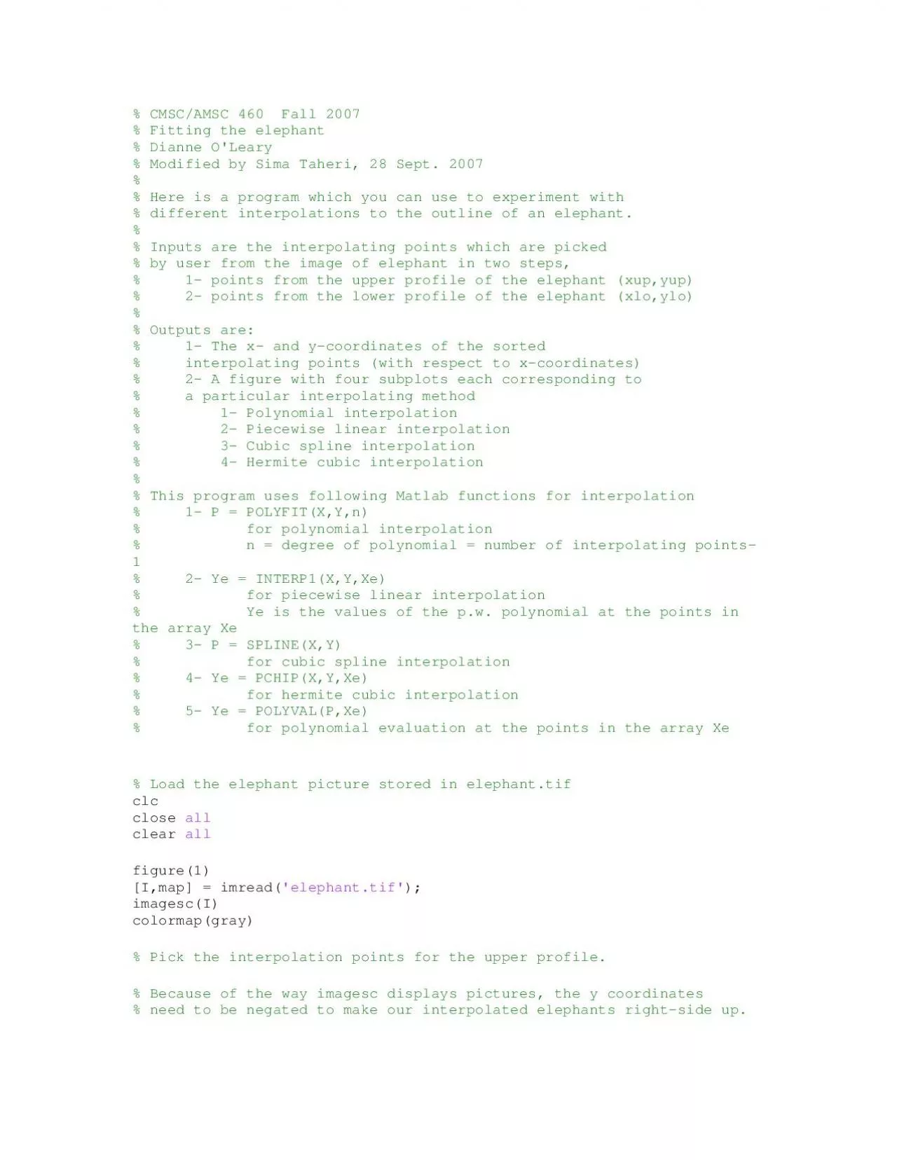
/
CMSCAMSC 460  Fall 2007  Fitting the elephant  Dianne OLeary CMSCAMSC 460  Fall 2007  Fitting the elephant  Dianne OLeary

CMSCAMSC 460 Fall 2007 Fitting the elephant Dianne OLeary - PDF document

arya
arya . @arya
Follow
342 views
Uploaded On 2021-06-30

CMSCAMSC 460 Fall 2007 Fitting the elephant Dianne OLeary - PPT Presentation

dispPick interpolation points for the upper profile of the elephant xupyup ginput yup yup Note that the xcoordinates must be in ascending order in order for ID: 850234

yup ylo xup xlo ylo yup xlo xup plot interpolation points xplot profile elephant upper kplot cubic spline hermite

Share:

Link:

Embed:

Download Presentation from below link

Download Pdf The PPT/PDF document "CMSCAMSC 460 Fall 2007 Fitting the ele..." is the property of its rightful owner. Permission is granted to download and print the materials on this web site for personal, non-commercial use only, and to display it on your personal computer provided you do not modify the materials and that you retain all copyright notices contained in the materials. By downloading content from our website, you accept the terms of this agreement.


Presentation Transcript

1 % CMSC/AMSC 460 Fall 2007 % Fitting the
% CMSC/AMSC 460 Fall 2007 % Fitting the elephant % Dianne O'Leary % Modified by Sima Taheri, 28 Sept. 2007 % % Here is a program which you can use to experiment with % different interpolations to the outline of an elephant. % % Inputs are the interpolating points which are picked % by user from the image of elephant in two steps, % 1- points from the upper profile of the elephant (xup,yup) % 2- points from the lower profile of the elephant (xlo,ylo) % % Outputs are: % 1- The x- and y-coordinates of the sorted % interpolating points (with respect to x-coordinates) % 2- A figure with four subplots each corresponding to % a particular interpolating method % 1- Polynomial interpolation % 2- Piecewise linear interpolation % 3- Cubic spline interpolation % 4- Hermite cubic interpolation % % This program uses following Matlab functions for inte

2 rpolation % 1- P = POLYFIT(X,Y,n) %
rpolation % 1- P = POLYFIT(X,Y,n) % for polynomial interpolation % n = degree of polynomial = number of interpolating points-1 % 2- Ye = INTERP1(X,Y,Xe) % for piecewise linear interpolation % Ye is the values of the p.w. polynomial at the points in the array Xe % 3- P = SPLINE(X,Y) % for cubic spline interpolation % 4- Ye = PCHIP(X,Y,Xe) % for hermite cubic interpolation % 5- Ye = POLYVAL(P,Xe) % for polynomial evaluation at the points in the array Xe % Load the elephant picture stored in elephant.tif clc close all clear all figure(1) [I,map] = imread('elephant.tif'); imagesc(I) colormap(gray) % Pick the interpolation points for the upper profile. % Because of the way imagesc displays pictures, the y coordinates % need to be negated to make our interpolated elephants right-side up. disp(

3 'Pick interpolation points for the upper
'Pick interpolation points for the upper profile of the elephant.') [xup,yup] = ginput; yup = - yup; %%%%%%%%%%%%%%%%%% % Note that the x-coordinates must be in ascending order in order % for the piecewise linear, the cubic spline and Hermite cubic fits to % be correct. Therefore, we sort the x-coordinates in ascending order. % Y = SORTROWS(X) sorts the rows of the matrix X in ascending order % % Sort the x-coordinates of the upper profile in ascending order InpUp = [xup,yup]; SInpUp = sortrows(InpUp); xup = SInpUp(:,1); yup = SInpUp(:,2); %%%%%%%%%%%%%%%%%% % Pick the interpolation points for the lower profile. disp('Pick interpolation points for the lower profile.') disp('The two endpoints from the upper will be reused.') [xlo,ylo] = ginput; ylo = -ylo; %%%%%%%%%%%%%%%% % Sort the x-coordinates of the lower profile in ascending order InpLo = [xlo,ylo]; SInpLo = sortrows(InpLo); xlo = SInpL

4 o(:,1); ylo = SInpLo(:,2); %%%%%%%%%%%%%
o(:,1); ylo = SInpLo(:,2); %%%%%%%%%%%%%%% % To connect the upper interpolation to the lower one reuse the % end points % By this way, we do not have inappropriate connection % between lower and upper interpolation polynomials if xup(1) xlo(1) xlo = [xup(1);xlo]; ylo = [yup(1);ylo]; else xup = [xlo(1);xup]; yup = [ylo(1);yup]; end if xup(end) � xlo(end) xlo = [xlo;xup(end)]; ylo = [ylo;yup(end)]; else xup = [xup;xlo(end)]; yup = [yup;ylo(end)]; end nup = length(xup); nlo = length(xlo); disp('Sorted interpolation points from the upper profile:') [xup,yup] disp('Sorted interpolation points from the lower profile:') [xlo,ylo] % Compute and evaluate the interpolating functions: xplot = linspace(min(xlo),max(xlo),100); xloe = xplot; xupe = xplot; figure(2) kplot = 1; npts = nlo + nup - 2; % First, the polynomial polyPup = polyfit(xup,yup,

5 nup-1); yup_poly = polyval(polyPup,xup
nup-1); yup_poly = polyval(polyPup,xupe); yup_plot = polyval(polyPup,xplot); polyPlo = polyfit(xlo,ylo,nlo-1); ylo_poly = polyval(polyPlo,xloe); ylo_plot = polyval(polyPlo,xplot); subplot(2,2,kplot) plot(xplot,yup_plot,xplot,ylo_plot) hold on plot(xlo,ylo,'*',xup,yup,'o') axis([0 400 max(-1000,min(ylo_plot)),min(500,max(yup_plot))]) pp = sprintf('Polynomial elephant, %d points',npts); title(pp) kplot = kplot + 1; % Next, the piecewise linear. % I chose to use the Matlab function interp1, but % using the book's functions would be fine. ylo_plot = interp1(xlo,ylo,xplot); yup_plot = interp1(xup,yup,xplot); ylo_lin = interp1(xlo,ylo,xloe); yup_lin = interp1(xup,yup,xupe); subplot(2,2,kplot) plot(xplot,yup_plot,xplot,ylo_plot) hold on plot(xlo,ylo,'*',xup,yup,'o') pl = sprintf('Piecewise linear elephant, %d points',npts); title(pl) kplot = kplot + 1; % the cubic

6 spline coef_lo = spline(xup,yup); coe
spline coef_lo = spline(xup,yup); coef_up = spline(xlo,ylo); ylo_plot = ppval(coef_lo,xplot); yup_plot = ppval(coef_up,xplot); ylo_spline = ppval(coef_lo,xloe); yup_spline = ppval(coef_up,xupe); subplot(2,2,kplot) plot(xplot,yup_plot,xplot,ylo_plot) hold on plot(xlo,ylo,'*',xup,yup,'o') cs = sprintf('Cubic spline elephant, %d points',npts); title(cs) kplot = kplot + 1; % Finally, the Hermite cubic, % Here I chose to use the pchip function in Matlab ylo_plot = pchip(xlo,ylo,xplot); yup_plot = pchip(xup,yup,xplot); ylo_Hermite = pchip(xlo,ylo,xloe); yup_Hermite = pchip(xup,yup,xupe); subplot(2,2,kplot) plot(xplot,yup_plot,xplot,ylo_plot) hold on plot(xlo,ylo,'*',xup,yup,'o') ch = sprintf('Hermit cubic elephant using pchip, %d points',npts); title(ch) % Here I chose to use the van Loan's software for % Hermite cubic interpolation % Find the derivative values at the interpolation p

7 oints up = (yup(2:end)-yup(1:end-1))./(
oints up = (yup(2:end)-yup(1:end-1))./(xup(2:end)-xup(1:end-1)); slo = (ylo(2:end)-ylo(1:end-1))./(xlo(2:end)-xlo(1:end-1)); sup = [sup;slo(end)]; slo = [sup(1);slo]; [alo,blo,clo,dlo] = pwC(xlo,ylo,slo); [aup,bup,cup,dup] = pwC(xup,yup,sup); ylo_plot = pwCEval(alo,blo,clo,dlo,xlo,xplot); yup_plot = pwCEval(aup,bup,cup,dup,xup,xplot); ylo_Hermite = pwCEval(alo,blo,clo,dlo,xlo,xloe); yup_Hermite = pwCEval(aup,bup,cup,dup,xup,xupe); ----------------------------------------------------------------- - Pick interpolation points for the upper profile of the elephant. Pick interpolation points for the lower profile. The two endpoints from the upper will be reused. Sorted interpolation points from the upper profile: ns = 33.6486 -122.6067 88.4159 -5.1477 261.3652 -4.3026 399.7247 -98.9459 orted interpolation points from the lower profile: ns = 33.6486 -122.6067 72.0818 -2

8 35.8406 97.0634 -114.1564 196.0288
35.8406 97.0634 -114.1564 196.0288 -278.9371 265.2085 -174.1535 318.0541 -275.5570 376.6647 -155.5629 399.7247 -98.9459 - ick interpolation points for the upper profile of the elephant. Pick interpolation points for the lower profile. The two endpoints from the upper will be reused. Sorted interpolation points for the upper profile: ns = 32.6878 -133.5921 91.2984 -5.9927 123.0058 -13.5980 161.4389 -7.6827 263.2869 -4.3026 338.2316 -27.9635 396.8422 -95.5658 orted interpolation points for the lower profile: ns = 32.6878 -133.5921 52.8652 -228.2354 71.1210 -235.8406 85.5334 -128.5219 112.4366 -109.9313 127.8099 -116.6915 169.1256 -279.7822 218.1279 -274.7120 245.9919 -170.7734 272.8952 -172.4635 294.0334 -273.0219 340.1532 -283.1623 356.4873 -277.2471 359.3698 -202.8845 387.2339 -124.2968 393.9597 -245.1360 396.8422 -95