Experimental economics John Hey - PowerPoint Presentation

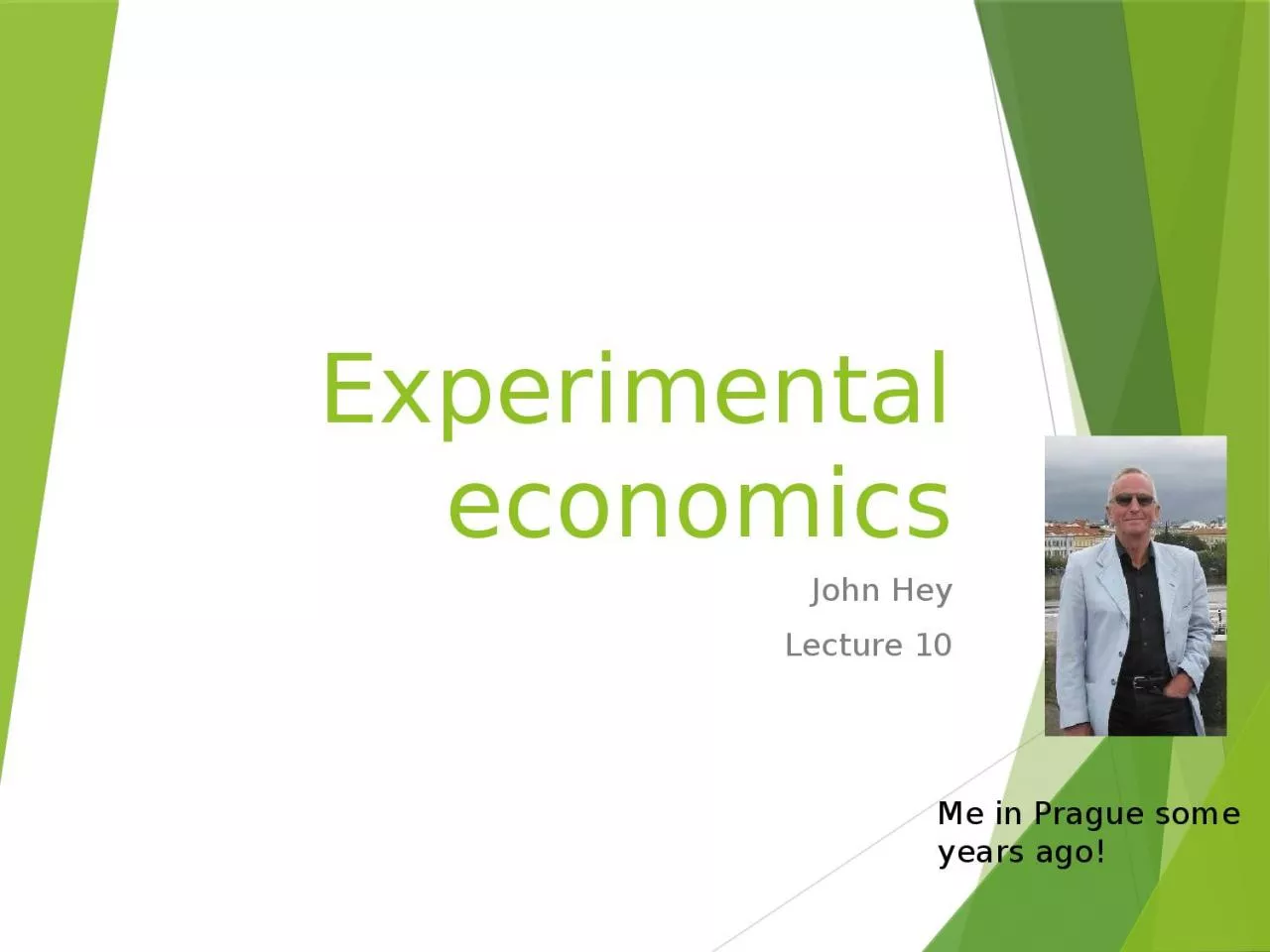
1. Experimental economicsJohn HeyLecture 10Me in Prague some years ago!

2. Individual experimentsI have decided to make the last lecture in this course (Lecture 12) a sort of general overview.In the lectures 10 and 11, I will talk about individual experiments.Lecture 10: Static decision-making under risk (and under ambiguity)Lecture 11: Dynamic decision-making

3. Decision-making under riskTheories – start with axioms.There are lots of theories based on different axioms.We can do two things:Test axioms and theories.Fit preference functionals.

4. Expected utility theorySays that decision-makers act on the basis of the utility that they expect to get.(If the utility function is linear in money, and the outcomes are money, they act on the basis of the return that they expect to get – risk neutrality.)It is based on axioms:CompletenessTransitivityIndependenceContinuity

5. EU axiomsBy a ‘(p-)mixture’ of two things, we mean a lottery which results in one of these things with probability p and the other with probability 1-p.Completeness: given any two things, the DM can always say that one or the other is preferred, or he or she is indifferent.Transitivity: If A is preferred to B and B preferred to C then A is preferred to C.Independence: If A is preferred to B then a mixture of A with C is preferred to the same mixture of B with C.Continuity: If A is preferred to B and B preferred to C then there must be a mixture of A and C for which there is indifference with B.

6. AxiomsEconomists love axioms – definitions of ‘rationality’.They are beautiful and intellectually appealing.Consider the Independence Axiom.Suppose you prefer A to B, where A and B can be anything.Now suppose you are offered the following risky choice: between Left and Right. Which would you choose? C is anything. p is anything.ACp1-pBCThese are both risky choices with probabilities p and 1-p.RightLeft

7. Now a testWhat would you choose here? And here?£300£0£4000.80.20.20.750.25Are your decisions consistent with the Independence Axiom?

8. Now a testWhat would you choose here?£300£0£4000.80.2And here?0.750.250.2Are your decisions consistent with the Independence Axiom?

9. This is the Allais ‘paradox’The Independence Axiom is the crucial part of Expected Utility theory. Experimental tests of this axiom and others have led to the development of new theories of behaviour under risk, most notably Prospect theory and Rank-Dependent Expected Utility theory.Allais (Nobel Prize 1988) was an early experimenter in the field.

10. The Marschak-Machina triangle01Used for portraying lotteries with 3 outcomes such that x1 preferred to x2 and x2 is preferred to x3. x1 is the outcome with probability p1, x2 is the outcome with probability p2 and x3 is the outcome with probability p3, Of course p1+ p2+ p3 = 1.

11. Indifference curves in the MMT for EUAn indifference curve is given byp1u(x1) + p2u(x2) + p3u(x3) = constant.Denoting u(xi) by ui, i=1,2,3 and using p1+ p2+ p3 = 1, we can write the equation of an indifference curve as:p1 = [(u2-u3)/ (u1-u2)]p3 + constant.This is an upward-sloping line in the MMT.

12.

13. A Common Ratio EffectProblem from above:(1) Do you prefer (A) £300 for sure, or (B) a lottery which yields £400 with probability 0.8 and £0 with probability 0.2?(2) Do you prefer (A) a lottery which yields £300 with probability 0.25 and £0 with probability 0.75, or (B) a lottery which yields £400 with probability 0.2 and £0 with probability 0.8?A preference for A in problem 1 and for B in Problem 2 is a violation of the Indpendence Axiom and hence of Expected Utility theory.

14. Common ratio effect in the mmt

15. Camerer (1989)

16.

17.

18.

19.

20. New Theories

21.

22.

23.

24.

25. Experimental detailsHow many subjects?Depends on how different people are.How many problems per subject?Depends upon how much noise in their behaviour.How should the problems be chosen?Depends what you want to test.How should the lotteries be presented?Might there be a ‘framing effect’?How would you do the playout?

26. Presentation of lotteries

27.

28. What I prefer now

29. Axioms and theoriesAll axioms are wrong.All more general theories fit better than less general theories that are nested inside them.Is this interesting or important?How wrong are they?How much better is the fit?Statistical significance just tells you that you have enough data.What is more crucial is economic significance.

30. Testing axioms or fitting preference functionals? Theories are composed from sets of axioms.Testing axioms enable us to discover which bits of theories are wrong.How many violations of an axiom are enough to condemn it?Fitting preference functionals enables us to see how well a theory fits the data.But fitting preference functionals requires the specification of functional forms and the estimation of parameters.Which is best?

31. Testing axioms experimentally – how?CompletenessTransitivityIndependenceContinuityAlmost all of these relate to relationships between gambles.The obvious way to start testing them is with pairwise choices – but these have to be specific.So not testing the axiom as a whole (unless by asking? Would that work?)How would one test the above axioms?

32. Estimating preference functionalsUp to now the literature was concerned with testing.In 1994 with the papers by Harless and Camerer and by Hey and Orme, the focus shifted to estimation.Fit preference functionals and see which fits best – taking into account degrees of freedom.

33. Hey and Orme (1995)Estimating preference functionals: RN, EU, DA, PR, QU, RD, RI, RP, RQ, WU and YD.80 subjects given 100 pairwise choice questions on two separate occasions.All lotteries led to one of £0, £10, £20, £30.Random lottery payment mechanism used on each occasion.

34.

35.

36. Stochastic assumptionsWe assumed that choice is made on the basis of the true preference function plus error – Normal with mean 0 and s.d. s.L stated as preferred to R if and only if V(L) – V(R) + e > 0. (For subjects never indifferent) What about indifference? Theshold t such that L and R stated as indifferent ift > V(L) – V(R) + e > -t.This is called the Random Utility Model (RUM)An alternative is the Random Preference Model (RPM)In this the parameter(s) r is/are random

37. EstimationAll the different preference functionals fitted/estimate using Maximum Likelihood.Parameters of the models (depends how you characterise the utility ‘function’) plus the stochastic parameters estimated.Models compared on the basis of their maximised log-likelihood corrected for degrees of freedom:Aikake Criterion.

38.

39. Harless and CamererThey pool observations from lots of subjects.They have a different error story – they assume that subjects state their preferred choice with a given probability.This is called the ‘Tremble Story’.Other error stories – for example, Loomes and Sugden assume stochastic preferences.

40. Recent workHey and Orme showed that “EU plus noise” is not a bad description of the data.Problems with non-violation of dominance.Clear that noise is not homoscedastic.Blavatskky shows that an appropriately specified heteroscedastic model (with EU) is pretty good.

41. Conclusions on riskIn a sense we have come full circle.The early tests of EU showed that it did not do too well......as a consequence lots of new models were formulated.These were then estimated and attention focussed on ‘noise’......with appropriately specified noise, “EU plus noise” is not too bad.

42. A DigressionDoes the elicitation mechanism affect the results?See Zhou and Hey Context Matters, Experimental Economics, online 2017.In this, we estimated the risk attitude of 96 subjects using 4 different elicitation methods:Holt-Laury Price Lists (48 such lists)Pairwise Choices (80 such pairs)The Becker-DeGroot-Marshak method (modified) 54 problemsAllocation problems (81 such problems)

43. Our Presentation of a lottery

44. Results –a summaryThe different elicitation methods produced widely divergent estimates of risk aversion. Some examples follow on the next slides (the scatters differ across the preference functional assumed).

45. Expected Utility with Constant Relative Risk AversionKey: HL: Holt Laury; PC:Pairwise Choice; LC: Becker-DeGroot Marschak; AL: Allocation

46. Our ConclusionContext Matters.

47. Behaviour under ambiguityRecent years have witnessed many new theories of behaviour under ambiguity (where objective probabilities do not exist or are not known).These are also based on axioms.Testing and estimating these are difficult, mainly because of the difficulty of implementing ambiguity in the laboratory.‘Ellsberg urns’ are difficult to implement because of subjects’ possible suspicion, and possible problems of the violation of ethical standards.We use a Bingo Blower…… which I will show you later.

48. Models of Behaviour under ambiguitySubjective Expected UtilityChoquet Expected UtilityCumulative Prospect TheoryMaxmin Expected Utilityα-maxmin Expected UtilityConfidence FunctionVariational PreferencesThe ‘Contraction’ ModelSmooth Ambiguity ModelSurvey in Etner et al Journal of Economic Surveys 2012.

49. Experiments I have conducted on AmbiguityHey. Lotito and Maffioletti JRU (2010), The Descriptive and Predictive Adequacy of Theories of Decision Making Under Uncertainty/AmbiguityHey and Pace JRU (2014), The Explanatory and Predictive Power of Non Two-Stage-Probability Models of Decision Making Under Ambiguity.Carbone, Dong and Hey, Elicitation of Preferences under Ambiguity, JRU (2017)

50. Hey. Lotito and MaffiolettiWe used the BBB.We had three treatments –with different amounts of ambiguity.Pairwise choice questions – between ambiguous gambles with payoffs -£10, £10 and £100 (with a show-up fee of £10). Random Payment mechanism

51. Let us suppose that you confront two urns containing red and black balls, from one of which a ball will be drawn at random. To "bet on Red I" will mean that you choose to draw from Urn I; and that you will receive a prize a (say $100) if you draw a red ball ("if Red I occurs") and a smaller amount b (say, $0) if you draw a black ("if not-Red I occurs"). You have the following information. Urn I contains 100 red and black balls, but in a ratio entirely unknown to you; there may be from 0 to 100 red balls. In Urn II, you confirm that there are exactly 50 red and 50 black balls. An observer – who, let us say, is ignorant of the state of your information about the urns – sets out to measure your subjective probabilities by interrogating you as to your preferences in the following pairs of gambles:"Which do you prefer to bet on, Red I or Black I: or are you indifferent?" That is, drawing a ball from Urn I, on which "event" do you prefer the $100 stake, red or black: or do you care?”"Which would you prefer to bet on, Red II or Black II?""Which do you prefer to bet on, Red I or Red II?""Which do you prefer to bet on, Black I or Black II?”This experiment was inspired by Ellsberg

52. Hey. Lotito and MaffiolettiThe following is a screenshot of one problem from the experiment.They were all pairwise choice questions

53.

54. The TreatmentsTreatment 1: 2 pink, 5 blue, 3 yellowTreatment 2: 4 pink, 10 blue, 6 yellowTreatment 1: 8 pink, 20 blue, 12 yellowIn Treatment 1, the balls can be counted.In Treatment 2, the pink can be counted and possibly the yellow but not the blue.In Treatment 3, no colour can be counted.

55.

56.

57.

58. The DesignParticipation fee of £10.3 colours (pink, blue and yellow) .3 amounts of money (-£10, £10 and £100).Pairwise choice questions.33 = 27 different lotteries and hence 27x26/2 = 351 possible pairwise choices.Omitting those with dominance leaves us with 162 pairwise choice questions.Order and left-right juxtaposition randomised.

59. The Preference Functionals No Multiple Prior ModelsSubjective Expected Utility (SEU)‘Prospect Theory’ (PT)Choquet Expected Utility (CEU)Cumulative Prospect Theory (CPT)Decision Field Theory (DFT) Gilboa and Schmeidler’s MaxMin Expected Utility theory (GS Min)Gilboa and Schmeidler’s MaxMax Expected Utility theory (GS Max)The Alpha EU Model (Ghiradarto et al)MaximinMaximaxMinimax RegretHurwicz Model

60. Estimation of Models All preference functionals parameterised.Stochastic Specifications:(1) For the models which have a preference functional we assume that preferences are measured with error such that the differences in the evaluations of the two lotteries is N(0, s2). We estimate s along with the other parameters.For the DFT model the errors are not homoscedastic but have a variance which depends on the lotteries.(2) For the other models, the not-preferred choice is implemented with probability w. We estimate w along with the other parameters.We estimated using Maximum Likelihood in GAUSSWe also used the data to predict (out-of-sample)

61. Conclusions 1We can dismiss CEU, CPT, Minimax Regret and the Hurwicz Criterion. GS Max is best only once and Alpha only one-and-a-half times. Of the remaining models, clearly the best are PT and DFT, while EU, GS Min, MaxMin and MaxMax score almost equally. As we go from Treatment 1 through Treatment 2 to Treatment 3, we note that there is a very slight evidence of an increase in the ‘rules of thumb’, MaxMin and MaxMax; also interestingly and counter-intuitively, EU seems to improve, with a corresponding decline in PT.

62. Conclusions 2The simpler models seem to do better.What about the Multiple Prior models?Many more parameters to estimate.There is an identification problem.Perhaps people prefer to simplify a complicated problem rather than apply a complicated decision rule?

63. Hey and PaceWe used the allocation method to elicit preferences (thinking it might be better than pairwise choices).

64. The Experiment64We asked the subjects a total of 76 questionsThere were two types of question: 1. The first type of question was to allocate a given quantity of tokens between two of the three colours in the Bingo Blower 2. The second type of question was to allocate a given quantity of tokens between one of the three colours in the Bingo Blower and the other two

65. The First Type of Question65In this type we gave the subject a given quantity of tokens and asked him or her to allocate them between two of the three colours in the Bingo BlowerThat is, between pink and blue, or between blue and yellow, or between yellow and pinkWe also told the exchange rate between tokens and money for each colourAn allocation of tokens between the two colours implies an amount of money for each of the two colours

66.

67. The Second Type of Question67In this type we gave the subject a quantity of tokens and asked him or her to allocate them between one of the three colours in the Bingo Blower and the other twoThat is, between pink and not-pink (that is, blue and yellow), or between blue and not-blue (that is, yellow and pink), or between yellow and not-yellow (that is, pink and blue)We also told the exchange rate between tokens and money for each colourAn allocation of tokens between the one colour and the other two implies an amount of money for the one colour and the other two

68.

69. Payment69At the end of the experiment, for each subject, one of the 76 questions was picked at randomThe subject then ejected one ball from the Bingo Blower (he or she could not manipulate the ejection)Its colour determined their payment, as we show in the following slides

70. Payment if this problem is selected at randomIf the ball ejected was yellow you would get paid £15.00, if the ball ejected was pink you would get paid £10.50 and if the ball ejected was blue you would get paid nothing

71. Payment if this problem is selected at randomIf the ball ejected was pink you would get paid £15.00, if the ball ejected was blue you would get paid £15.00 and if the ball ejected was yellow you would get paid £12.00

72. 72Result: Precision increasesPARAMETER OF PRECISIONFirst 38 QLast 38 Qt-stat diffOverall12.81815.320-3.068Treatment 113.68716.100-2.505Treatment 211.90914.502-1.939 Precision increases significantly during the experiment, expecially in Treatment 1 (less ambiguous)

73. 73 First 38 QLast 38 Qt-stat diffSEUTreatment 112.79615.028-2.542Treatment 211.29113.495-1.748    CEUTreatment 113.98516.711-2.760Treatment 212.18814.690-1.844    AEUTreatment 113.82716.508-2.668Treatment 212.02415.017-2.111    VEUTreatment 114.67816.937-1.960Treatment 212.67415.727-2.108    COMTreatment 113.14815.318-2.390Treatment 211.36713.583-1.725Result: Precision increases

74. 74Result: Risk Aversion does not change RISK AVERSIONFirst 38 QLast 38 Qt-stat diffOverall0.7950.799-0.251Treatment 10.7940.815-1.078Treatment 20.7960.7830.444 The changes are not statistically significant

75. 75 First 38 QLast 38 Qt-stat diffSEUTreatment 10.8000.817-0.863Treatment 20.8030.7890.512    CEUTreatment 10.8000.817-0.797Treatment 20.7970.7730.818    AEUTreatment 10.7850.810-1.270Treatment 20.7880.7790.313    VEUTreatment 10.7830.808-1.314Treatment 20.7790.7780.060    COMTreatment 10.8030.819-0.868Treatment 20.8040.7890.507Result: Risk Aversion does not change

76. 76Results Test for CEU: Additivity of capacities REJECTED Test for AEU: Additivity of probabilities and lower ambiguity aversion REJECTED Test for VEU: lower ambiguity aversion REJECTED Test for COM: Additivity of probabilities and lower ambiguity aversion REJECTED

77. Carbone, Dong and HeyThis was expressed as a Portfolio Choice Problem.Subjects were asked to allocate 100 tokens to 3 assets with stated rates of return.

78. Portfolio Choice Problem Decision Maker (DM) has 100 to allocate between cash and assets 1 and 2 Allocations: c1, c2, and c0=100- c1- c2Portfolio Payoff : dj=c0 +r1,jc1+r2,jc2, (in state j=1,2,3)78State 1State 2State 3Asset 1r11r12r13Asset2r21r22r23

79. ConclusionsMV did rather badly SEU does quite well Subjects do not use a more complicated preference functional when choosing allocations in a complicated settingSF worse than SEU Some sophistication in decision making

80. Conclusions on experiments on ambiguityThe overall conclusion must be that the sophisticated theories of behaviour under ambiguity are too sophisticated for human beings.

81. That is the end of lecture 10.Phew!! ‘See you’ next week.