/
Optimizing Riparian Optimizing Riparian

Optimizing Riparian - PowerPoint Presentation

calandra-battersby
calandra-battersby . @calandra-battersby
Follow
406 views
Uploaded On 2017-09-14

Optimizing Riparian - PPT Presentation

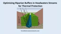
Buffers for Thermal Protection TerrainWorks wwwterrainworkscom We ask the question What is the optimum design and width of riparian buffers to protect against increases in thermal energy and how does that compare to fixed ID: 587772

width buffer fixed protection buffer width protection fixed optimized channel density buffers thermal left area streams 100 azimuth stream radiation riparian based

Share:

Link:

Embed:

Download Presentation from below link

Download Presentation The PPT/PDF document "Optimizing Riparian" is the property of its rightful owner. Permission is granted to download and print the materials on this web site for personal, non-commercial use only, and to display it on your personal computer provided you do not modify the materials and that you retain all copyright notices contained in the materials. By downloading content from our website, you accept the terms of this agreement.


Presentation Transcript

Slide1

Optimizing Riparian Buffers for Thermal Protection

TerrainWorks

(www.terrainworks.com)Slide2

We ask the question:What is the optimum design and width of riparian buffers to protect against increases in thermal energy and how does that compare to fixed

with buffers in headwater streams?Slide3

To answer that question, we employ NetMap’s “virtual watershed” that evaluates thermal load that is sensitive to solar angle, latitude, topography,

channel width, channel orientation and streamside vegetation height and density.Slide4

Most thermal buffer rules are based on policy negotiations aimed at balancing thermal

protection with forest economic values (timber harvest). Regardless of policy negotiations,most buffer width dimensions are based on studies and literature that have identified

threshold buffer widths using stream temperature field measurements and or modeling.

The general rule of thumb is that buffers between 75 and 100 feet are necessary to ensure

thermal loading protection. In general, no consideration is given to stream orientation that

strongly influences thermal energy to streams, including left and right side of the channel.

Field studies that identify buffer width thresholds cannot, for practical reasons, consider

the full variability of channel characteristics.Here, we use a thermal energy calculation to help understand the design of optimized bufferwidths.

BackgroundSlide5

Project area:

Teanaway

River watershed

in the Yakima River basin, eastern

Washington; analysis limited to

non fish bearing streams less than

10 km

2 (2470 acres) in area.Study AreaSlide6

In the Teanaway River watershed in eastern Washington, we compare a few different riparian

buffer designs on headwater, non fish bearing streams (approx. 14,370,

100 m reach segments):

Optimized buffer widths that maximizes thermal energy reductions and that differentiates

right and left sides of channels (looking downstream

) and accounts for varying azimuth,

Fixed with buffers at widths of 25

ft, 50 ft, 75 ft and 100 ft (same on both sides of the

channel);

We use a density of riparian forests of 70% (can be varied)

to

calculate light

transmission using a physically based model of thermal loading; the model incorporates

“Beers Law”,

a

common

approach in

thermal

loading models

(density is a function of leaf area index,

DeWalle

2010)

.

DeWalle

, D. 2010. Modeling stream shade: riparian buffer height and density as important as buffer width. Journal of American Water Resources Association. 1-11:1752-1688.Slide7

Channel direction or azimuth

(0 – 360

deg

) matters:

N-S oriented streams require similar

buffer widths on both sides of the

stream;

whereas, E-W oriented streams haveless buffer width on the north sideof the channel.Slide8

The attenuation of solar

radiation with buffer

width is governed by

a power law (Beers Law)

less and less light radiation

comes into the stream

with increasing distance

from the stream withina bufferSlide9

There is a rapidly diminishing

effectiveness of increasing

buffer width on radiation

protection (sketch)Slide10

Optimized buffers - analysis approach

1) calculate bare Earth radiation (

maximum),

2) calculate

maximum

possible radiation

reduction or protection

(500 m forest width, density = 0.7),3) specify a percent reduction in radiation (25%, 50%, 75%, 90%, 95%, 99%) between bare Earth and the maximum

reduction.

Bare Earth

Maximum

reduction

Specify % protection

Example – 90%

X

ftSlide11

Here is a mapped example of

model outputs:

Optimized

buffers are less

wide on the north sides of streams

along east – west flowing channels

little difference in north – sound

trending streamsSlide12

The next three slides illustrate the effects of stream orientation (azimuth) on left and right buffers at three levels of thermal loading protection:80%, 90% and 99%; observe the y axis differences in left-right buffer widthsSlide13

Optimized Buffer width (left-right) versus channel azimuth (80% protection)

Average tree

ht

= 25 m (82

ft

); density = 0.7Slide14

Optimized Buffer width (left-right) versus channel azimuth (90

% protection)

Average tree

ht

= 25 m (82

ft

); density = 0.7Slide15

Optimized Buffer width (left-right) versus channel azimuth (99

% protection)

Average tree

ht

= 25 m (82

ft

); density = 0.7Slide16

Prescription

Protection (%)

Area (acres)

Percent change

of fixed width area to optimized

buffer areas at 95%, 98% and 99%, respectively

Optimized, Left-right

95% 98% 99%

6,780 9,315 11,228

+37% +65%

Fixed width 25

ft

91%

5,219

-

23%

1

-43% -53%

Fixed width 50

ft

98%

10, 428

+54% +12% -7%

Fixed width 75

ft

99.7%

15,657

+130% +68% +39%

Fixed width 100

ft

99.9%

20,874

+207% +124% +86%

Comparison of optimized versus fixed with buffers, percent protection

and area required

1

((5,219-6,780)/5,219)*100Slide17
Slide18

Prescription

Protection (%)

Area (acres)

Percent change of fixed width area to optimized

buffer areas at 95%, 98% and 99%, respectively

Optimized, Left-right

95% 98% 99%

6,780 9,315 11,228

+37% +65%

Fixed width 25

ft

91%

5,219

-23% -43% -53%

Fixed width 50

ft

98%

10, 428

+54% +12% -7%

Fixed width 75

ft

99.7%

15,657

+130% +68% +39%

Fixed width 100

ft

99.9%

20,874

+207% +124% +86%

Matching an optimized buffer design to a protection level equal to that of a fixed width 50

ft

buffer decreases the

area under the buffer by 12% and ensures that 98% is the minimum protection – under the fixed 50ft, there

will be reaches that will not meet that minimum protection (e.g., protection improvement)

Comparing an optimized buffer to a fixed width 50

ft

buffer

1

((10,428-9,315)/9,315)*100

1Slide19

The optimized left-right buffer with a protection equivalent to a fixed 50

ft

bufferSlide20

The amount of thermal protectionafforded by incrementally increasing buffer

width rapidly diminisheswith increasing absolute buffer width and the area

encompassed by the buffer.Slide21

Predicted buffer width vs % protection is very sensitive to vegetation density term; reducing vegetationdensity to 0.50 yields 90% reduction for a 50ft buffer (rather than

98% with a 0.7 density) and a 75 ft and

100

ft

buffer yields only 93.5% and 94% protection; the key here is to determine what the “natural” density of

the riparian forest vegetation is and then use that as the baseline for all analyses and resulting buffer

prescriptions (changing vegetation density will not change the results shown in this PPT).Slide22

Possible buffer strategies:optimized (designer) buffers, select % protection, by tree height

and density – left, right buffer dimensions vary by channel segment azimuth etc. – create channel maps of optimized protection, apply reach by reach;

use

optimized

buffers to match some level of fixed

with buffer

protection (which will increase the effectiveness

above many fixed with buffers, for example, the 50 ft fixed with buffer shown in this PPT);for headwater non fish streams, select % protection based on probability of being seasonal vs non seasonal;

GIS based analysis will never be truly accurate with regards to channel orientation, channel width and tree height –

thus build a field based approach using a Tablet and or collect field data and re-calculate in the office (see next).Slide23

Improve accuracy

of optimized buffer

designsSlide24

Contact us for further information (www.terrainworks.com)