PDF-Seber Models

Author : calandra-battersby | Published Date : 2016-06-18

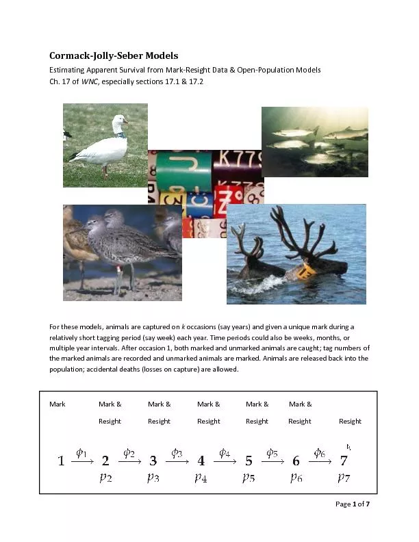
Page 1 of 7 Cormack Jolly Estimating Apparent Survival from Mark Resight Data Open Population Models Ch 17 of WNC especially sections 171 172 For these models

Presentation Embed Code

<iframe width="560" height="315" src="https://www.docslides.com/embed/366621" frameborder="0" allowfullscreen></iframe>

Download Presentation

Download Presentation The PPT/PDF document "Seber Models" is the property of its rightful owner. Permission is granted to download and print the materials on this website for personal, non-commercial use only, and to display it on your personal computer provided you do not modify the materials and that you retain all copyright notices contained in the materials. By downloading content from our website, you accept the terms of this agreement.

Seber Models: Transcript

Download Document

Here is the link to download the presentation.
"Seber Models"The content belongs to its owner. You may download and print it for personal use, without modification, and keep all copyright notices. By downloading, you agree to these terms.