/
The Art and Science of Mathematical Modeling The Art and Science of Mathematical Modeling

The Art and Science of Mathematical Modeling - PowerPoint Presentation

ceila
ceila . @ceila
Follow
66 views
Uploaded On 2024-01-03

The Art and Science of Mathematical Modeling - PPT Presentation

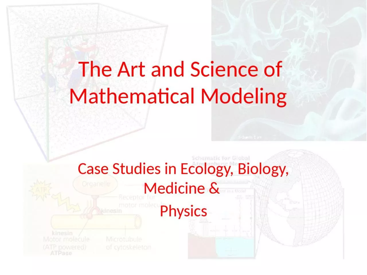
Case Studies in Ecology Biology Medicine amp Physics Prey Predator Models 2 Observed Data 3 A verbal model of predatorprey cycles Predators eat prey and reduce their numbers Predators go hungry and decline in number ID: 1036966

prey model modeling predator model prey predator modeling huxley hodgkin hiv predators time inhibitors neuron term number species deriving

Share:

Link:

Embed:

Download Presentation from below link

Download Presentation The PPT/PDF document "The Art and Science of Mathematical Mode..." is the property of its rightful owner. Permission is granted to download and print the materials on this web site for personal, non-commercial use only, and to display it on your personal computer provided you do not modify the materials and that you retain all copyright notices contained in the materials. By downloading content from our website, you accept the terms of this agreement.


Presentation Transcript

1. The Art and Science of Mathematical Modeling Case Studies in Ecology, Biology, Medicine & Physics

2. Prey Predator Models2

3. Observed Data3

4. A verbal model of predator-prey cycles:Predators eat prey and reduce their numbersPredators go hungry and decline in numberWith fewer predators, prey survive better and increaseIncreasing prey populations allow predators to increase ...........................And repeat…4

5. Why don’t predators increase at the same time as the prey?5

6. Simulation of Prey Predator System

7. 7The Lotka-Volterra Model: AssumptionsPrey grow exponentially in the absence of predators.Predation is directly proportional to the product of prey and predator abundances (random encounters).Predator populations grow based on the number of prey. Death rates are independent of prey abundance.

8. Generic Model f(x) prey growth term g(y) predator mortality term h(x,y) predation term e prey into predator biomass conversion coefficient

9. 9

10. Lotka-Volterra Model Simulations

11. 1 – no species can survive2 – Only A can live3 – Species A out competes B4 – Stable coexistence5 – Species B out competes A6 – Only B can live

12. Hodgkin Huxley ModelHow Neurons Communicate

13. Neurons generate and propagate electrical signals, called action potentialsNeurons pass information at synapses:The presynaptic neuron sends the message.The postsynaptic neuron receives the message.Human brain contains an estimated 1011 neurons Most receive information from a thousand or more synapses There may be as many as 1014 synapses in the human brain.

14. Neuronal CommunicationTransmission along a neuron

15. Action Potential How the neuron ‘sends’ a signal

16. Hodgkin Huxley Model –Deriving the Equations

17. Hodgkin Huxley Model –Deriving the Equations

18. Hodgkin Huxley Model

19. Hodgkin Huxley Model –Deriving the Equations

20. Hodgkin Huxley Model

21.

22. HIV : Models and Treatment

23. Modeling HIV InfectionUnderstand the processWorking towards a cureVaccination?

24. The Process

25. Lifespan of an HIV InfectionPoints to Note: Time in YearsT-Cell count relatively constant over a week

26. HIV Infection Model (Perelson- Kinchner)Modeling T-Cell Production:Assumptions:Some T-Cells are produced by the lymphatic systemOver short time the production rate is constantAt longer times the rate adjusts to maintain a constant concentrationT-Cells are produced by clonal selection if an antigen is present but the total number is boundedT-Cells die after a certain time

27. Modeling HIV Infection

28. Models of Drug Therapy – Line of AttackR-T Inhibitors: HIV virus enters cell but can not infect it.Protease Inhibitors: The viral particle made RT, protease and integrase that lack functioning .

29. RT Inhibitors (Reduce k!)A perfect R-T inhibitor sets k = 0:

30. Protease Inhibitors

31. Modeling Water Dynamics around a Protein

32. Multiple Time Scaleswww.nyu.edu/pages/mathmol/quick_tour.html

33. The SetupWant to study functioning of a protein given the structureBehavior depends on the surrounding moleculesExplicit simulation is expensive due to large number of solvent molecules

34. The General Program

35. Model IWe guess that behavior is captured by the drift and the diffusivity is the bulk diffusivityUse the following modelSimulate using Monte Carlo methodsCalculate the ‘bio-diffusivity’ and compare with MD results

36. Input to the model

37. Results from Model IModel does a poor job in the first hydration shell

38. Model IIWe consider a more general drift diffusion modelRun Monte Carlo Simulations and compare results with Model I

39. ComparisonModel II does a better job than Model I

40. Moral of the StoryMathematical models have been reasonably successful Applications across disciplinesChallenges in modeling, analysis and simulationYES YOU CAN!!!!

41. Questions??