PDF-ERROR PROPAGATION MODELINGJinda Sae-Jung, Xiao Yong Chen, Do Minh Phuo

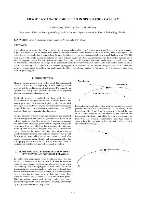
First select the point intersec 825 The International Archives of the Photogrammetry Remote Sensing and Spatial Information Sciences Vol XXXVII Part B2 Beijing 2008 Figure 1 Concept of model. Concern?. The unconscious but much broader. Insight?. Are patterns of growth that need to be made conscious. Central Problem?. Projection. Once unconscious want to become conscious it is projected onto world and others: unconscious evil within is projected onto others. Philip L. Bulterys,. 1. . T. huy. Le,. 2,3. . V. o . M. inh . Q. uang,. 4. . K. enrad E. Nelson,. 5. . J. ames O. Lloyd-Smith. 6,7. . 1. UCLA-Caltech Medical Scientist Training Program, David Geffen School of Medicine, University of California Los Angeles, Los Angeles, . Software Engineering Institute. Carnegie Mellon University. Pittsburgh, PA 15213. Peter H. Feiler. Jan 24, 2013. Copyright 2012 Carnegie Mellon University and IEEE. This . material is based upon work funded and supported by the Department of Defense under Contract No. FA8721-05-C-0003 with Carnegie Mellon University for the operation of the Software Engineering Institute, a federally funded research and development center.. An introduction to learning internal representations By error Propagation. Presented by:. Kunal Parmar. UHID: 1329834. 1. Outline of the Presentation. Introduction. Historical Background. Perceptron. Papa Jung!. Papa . jung. says,. “Who looks outside, dreams; who looks inside, awakes.”. Differences Between Freud and Jung. Most of Jung's assumptions of his analytical psychology reflect his . theoretical differences with Freud.  . He jumped out of bed and dressed quickly. He looked out the window to see if . Bao. was in the yard, but she was nowhere to be seen. Hearing his mother bustling in the kitchen, he went downstairs, his stomach telling him it was time for breakfast.. Oswaldo. Carrillo. Ruth Yanai. The State University of New York. Visit our website: . www.quantifyinguncertainty.org. Download papers and presentations. Share sample code. Stay updated with QUEST News. Schematic Modifications. Level Shifter. Level Shifter. Without level shifters, envelope detector output does not overlap with full input range of log amp. Level shifters increase correction range.. Psychology 209. February 6, 2013. Homework . 4. Part 1 due Feb 13. Complete . Exercises 5.1 and 5.2.. It may be helpful to . c. arry . out some explorations of parameters, as suggested in Exercise . 5.3. This may help you achieve a solution in the last part of the homework, below. However, no write-up is required for this.. Who has had the most positive influence on you?. 2. Give a name to the era we live in today (examples include the Hip-Hop Era, the Violent Generation, the New Baby Boomers, the Anti-Depression Era).. A Constraint Propagation Perspective. Rina . Dechter. Bozhena. Bidyuk. Robert. Mateescu. Emma. Rollon. Distributed Belief Propagation. Distributed Belief Propagation. 1. 2. 3. 4. 4. 3. 2. 1. 5. 5. 5. What are they?. Inspired by the Human Brain.. The human brain has about 86 Billion neurons and requires 20% of your body’s energy to function. . These neurons are connected to between 100 Trillion to 1 Quadrillion synapses!. The elaboration of this paper derived from a project supported first by the National Science Council NSC 92-2411-H-007-017 and later by the Boost Project at Tsing Hua University The author would like Significant Figures. Unit Conversion. Normal Distribution. Standard Deviation. Reading Error. Propagation of Errors. Error in the Mean. What is the approximate density of water?. 10. −5 . kg/m. 3.