PDF-Financial Market Anomalies Financial market anomalies PDF document

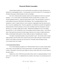
The term anomaly can be traced to Kuhn 1970 Documentation of anomalies often presages a transiti onal phase toward a new paradigm Discoveries of financial market

Upload by celsa-spraggs
Published on 2015-04-29

Presentation Embed Code

<iframe width="560" height="315" src="https://www.docslides.com/embed/56491" frameborder="0" allowfullscreen></iframe>

Download Presentation

Download Presentation The PPT/PDF document "Financial Market Anomalies Financial mar..." is the property of its rightful owner. Permission is granted to download and print the materials on this web site for personal, non-commercial use only, and to display it on your personal computer provided you do not modify the materials and that you retain all copyright notices contained in the materials. By downloading content from our website, you accept the terms of this agreement.