/
SYMBOLIC CALCULATION SYMBOLIC CALCULATION

SYMBOLIC CALCULATION - PDF document

celsa-spraggs
celsa-spraggs . @celsa-spraggs
Follow
402 views
Uploaded On 2016-08-10

SYMBOLIC CALCULATION - PPT Presentation

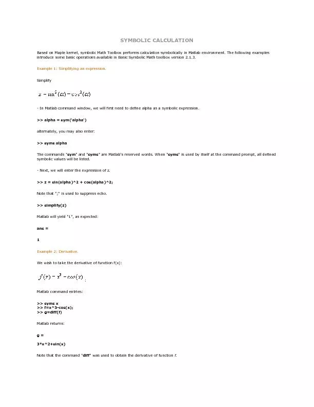
Based on Maple kernel symbolic Math Toolbox performs calculation symbolically in Matlab environment The following examples introduce some basic operations available in Basic Symbolic Math toolbox v ID: 441429

Based Maple kernel symbolic

Share:

Link:

Embed:

Download Presentation from below link

Download Pdf The PPT/PDF document "SYMBOLIC CALCULATION" is the property of its rightful owner. Permission is granted to download and print the materials on this web site for personal, non-commercial use only, and to display it on your personal computer provided you do not modify the materials and that you retain all copyright notices contained in the materials. By downloading content from our website, you accept the terms of this agreement.


Presentation Transcript

SYMBOLIC CALCULATION Based on Maple kernel, symbolic Math Toolbox performs calculation symbolically in Matlab environment. The following examples introduce some basic operations available in Basic Symbolic Math toolbox version 2.1.3. Example 1: Simplifying an expression. Simplify - In Matlab command window, we will first need to define alpha as a symbolic expression. �� alpha = sym('alpha') alternately, you may also enter: �� syms alpha The commands " sym " and " syms " are Matlab's reserved words. W hen " syms " is used by itself at the command prompt, all defined symbolic values will be listed. - Next, we will enter the expression of z. �� z = sin(alpha)^2 + cos(alpha)^2; Note that ";" is used to suppress echo. �� simplify(z) Matlab will yield "1", as expected: a ns = 1 Example 2: Derivative. We wish to take the derivative of function f(x): : Matlab command entries: �� syms x �� f=x^3 - cos(x); �� g=diff(f) Matlab returns: g = 3*x^2+sin(x) Note that the command " diff " was used to obtain the derivative of function f . Since function f has only one independent variable, the diff command performed the calculation based on x. If there are more than one independent variable in a function, you should include the "intended" v ariable in the following format: diff(f, x) where x is the "intended" variable. For example, We wish to obtain the derivative of the following function Matlab command entries: �� syms x y �� f=x^2+(y+5)^3; �� diff(f,y) Matlab returns: ans = 3*(y+5)^2 Note that in this case, the command diff(f,y) is equivalent to Example 3: Integral To integrate function f(x,y) as shown in Example 2, we will use the command " int " as shown below. �� int(f,x) Matlab returns: ans = 1/3*x^3+(y+5)^3*x The syntax of the integral command can be viewed by typing �� help int in Matlab command window. If we wish to perform the following definite integral: Matlab command entry: �� int(f,y,0,10) Matlab returns: ans = 12500+10*x^2 Example 4: Finding roots. Consider the following polynomial: Suppose we wish to find the roots of this polynomial. In Matlab Command window: �� syms x �� f=2*x^2 + 4*x - 8; �� solve(f,x) Matlab returns: ans = 5^(1/2) - 1 - 1 - 5^(1/2) Alternately, you may use the following lines in Mat lab to perform the same calculation: �� f=[2 4 - 8]; �� roots(f) Matlab returns: ans = - 3.2361 1.2361 Note that the results from both approaches are the same. Example 5: Matrix Symbolic Calculation This example demonstrates how Matlab handles matrix calcu lation symbolically. First we need to define the symbolic variables: �� syms a b c d e f g h Matrix A is then defined as: �� A=[a b; c d] Matlab's echo: A = [ a, b] [ c, d] Next, matrix B is defined as: �� B=[e f;g h] Matlab's echo: B = [ e, f] [ g, h] The addition of these two matrices yields: �� C=A+B C = [ a+e, b+f] [ c+g, d+h] and the product of A and B is: �� D=A*B D = [ a*e+b*g, a*f+b*h] [ c*e+d*g, c*f+d*h] If we wish to evaluate a specific matrix numerically, we simply assign the numeric values to the appropriate variable then us e the command eval as demonstrate below. �� a=1;b=2;c=3;d=4;e=5;f=6;e=7;f=8;g=9;h=0; �� eval(A) ans = 1 2 3 4 �� eval(B) ans = 7 8 9 0 �� eval(C) ans = 8 10 12 4 The inverse of A can be expressed symbolically: �� D=inv(A) D = [ d/(a*d - b*c), - b/(a*d - b*c)] [ - c/(a*d - b*c), a/(a*d - b*c)] Numerically, D is expressed by �� Dn=eval(inv(A)) Dn = - 2.0000 1.0000 1.5000 - 0.5000 As a verificati on, we may evaluate D directly: �� De=eval(D) De = - 2.0000 1.0000 1.5000 - 0.5000 You may also try �� Df=inv(eval(A)) to verify if you get the same result.