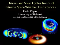
Extreme Space Weather Disturbances Emilia Kilpua University of Helsinki emiliakilpuahelsinkifi EmiliaKilpua Key solar wind parameters magnetic field magnitude and direction density ID: 559484
Download Presentation The PPT/PDF document "Drivers and Solar Cycles Trends of" is the property of its rightful owner. Permission is granted to download and print the materials on this web site for personal, non-commercial use only, and to display it on your personal computer provided you do not modify the materials and that you retain all copyright notices contained in the materials. By downloading content from our website, you accept the terms of this agreement.
Slide1
Drivers and Solar Cycles Trends of Extreme Space Weather Disturbances
Emilia Kilpua
University of Helsinki
(emilia.kilpua@helsinki.fi
@
EmiliaKilpua
)Slide2
Key solar wind parameters
magnetic field magnitude and direction
density
speed
level of turbulence
Alfvén
Mach
number (bow shock compression, how plasma flows around the magnetopause, saturation)
dawn
-dusk
(driving) electric field
d
ynamic pressureSlide3
highest
M
A
lowest M
A
p
olar cap potential
s
olar wind driving electric field (mV/m)
Solar wind
Alfvèn
Mach number and saturation
Myllys
et al., 2016Slide4
Effect of dynamic pressure
s
olar wind driving electric field (mV/m)
dynamic pressure (
nPa
)
p
olar cap potential
Myllys
et al., in preparationSlide5
Drivers of
geospace storms four Solar Cycles (1963 -2011)
G1 G2 G3 G4 G5
Coronal Mass Ejections (CMEs) drive nearly all intense
geospace
storms
Richardson and Cane
, 2012
Storm intensity:
Kp
(NOAA scales)Slide6
F
lux Rope
Sheath
Shock
Two principal CME structuresSlide7
Only flux ropes and sheaths have strong enough fields to drive extreme storms
Flux rope
S
heath
CIR
F
ast stream
Normalized occurrence distribution for events in 1997-2014Slide8
Sheaths have clearly higher
Pdyn and
Alfvén Mach number than flux ropes
Flux rope
S
heath
CIR
F
ast streamSlide9
Which CMEs drive the most extreme storms?
intrinsic CME properties
m
odifications during the IP journey
p
re-conditioning of the
heliosphere
“PERFECT STORM SCENARIO”
(
Liu et al
., 2014; 2015)Slide10
Nov 20, 2003 (Strongest
Dst storm of SC 23) driven by “isolated” CMESlide11
November 2001 storm and Halloween storms
impulsive energy injection
Balan et al
., JGR, 2014
V [km/s]
P
dyn
[
nPa
]
B
Z
[
nT
]
Dst
[
nT
]
> 60
nPaSlide12
prevents CME expansion CME maintains high fields and speeds
t
urbulent and compressed regions (high
P
dyn
and
M
A
)
shock merging (e.g.,
Lugaz
et al., 2015) and shock compression of the preceding ICME (e.g., Lugaz 2016: Statistical analysis based on the Heliospheric
S
hock Database
ipshocks.fi)
Liu et al., Nat Comm., 2014
CME-CME interactions Slide13
V
[
km/s]
n
[
nPa
]
“CME Sandwich”
(March 17, 2015)
Interactions with the other large-scale solar wind structures (CIR, fast stream, HPS)
Kataoka
et al
., GRL, 2015
c
ompresses sheath
and
FR
stronger storm than expected
F
ast stream compression enhances
geoeffectivity
of flux ropes with north-south rotating fields
(see e.g.,
Kilpua et al
.,
Ann.
Geophys
. 2012 and
Fenrich
&
Luhmann
, GRL, 1998)
f
ast
stream
FR
s
heath
B
[
nT
]
B
Z
[
nT
]
Dst
HPS
4
daysSlide14
low density
minimal drag force CME maintains high speeds
large
Ey
and stronger field line draping in the sheath
Liu et al.
, 2014
Preconditioning of the
heliosphere
l
ow density
p
revious weaker CMESlide15
Extreme Substorms
Extreme substorms
strong ionospheric
currents without significant ring current (Dst) storm (
Huttunen
and
Koskinen
, 2004;
Tsurutani
et al., 2015)
During CME sheath regions (Huttunen and Koskinen 2004)
Triggered by pressure pulses? (Tsurutani et al., 2015)
Strongest GICs occur during CME sheath regions (
Huttunen et al., Space Weather, 2008)Slide16
Strong Van
Allen belt enhancements: Fast streams are important
Kilpua et al., GRL, http://adsabs.harvard.edu
/abs/2015GeoRL..42.3076K, 2015Slide17
Occurrence of extreme storms
Carrington storm
July 22 “super-CME”Slide18
Correlation between solar cycle size and storm occurrence
Pearson correlation
coefficients, confidence intervals calculated with the bootstrap method. From
Kilpua et al., APJ, 2015
mean SSN
m
ax SSN
(14 cycles, SCs 11-23)
95%
confidence
correlation
between the
storm occurrence
and the
solar
cycle strength decreases with increasing storm magnitudeSlide19
Solar cycle phases and storms
Kilpua et al., APJ 2015Slide20
Weaker storms occur predominantly in the declining phase
(see also e.g., Ruzmaikin and
Feynmann, 2001)
poloidal
field
coronal holes CIRs and fast
streams
Stronger storms clustered close to maximum time
toroidal
field active regions coronal mass ejection (also probability for CME-CME interactions increases)Solar cycle phases and stormsSlide21
Summary
Extreme storms: strong (+ a few hours) BS, high
V, P
dyn and M
A
CME sheaths and interacting CMEs
“ Perfect Storm Scenario”: Strong and fast CME(s), favorable modifications during IP journey, pre-conditioning
Extreme space weather may occur also during weaker solar cycles (probability of the next Carrington storm?
Riley
2012: 10-yr occurrence probability 12%)
smaller-scale dynamo and turbulent fields? Stronger storms occur more near solar maximum