PDF-Does trader leverage exacerbate the liquidity comovement that we obser

Author : edolie | Published Date : 2021-08-25

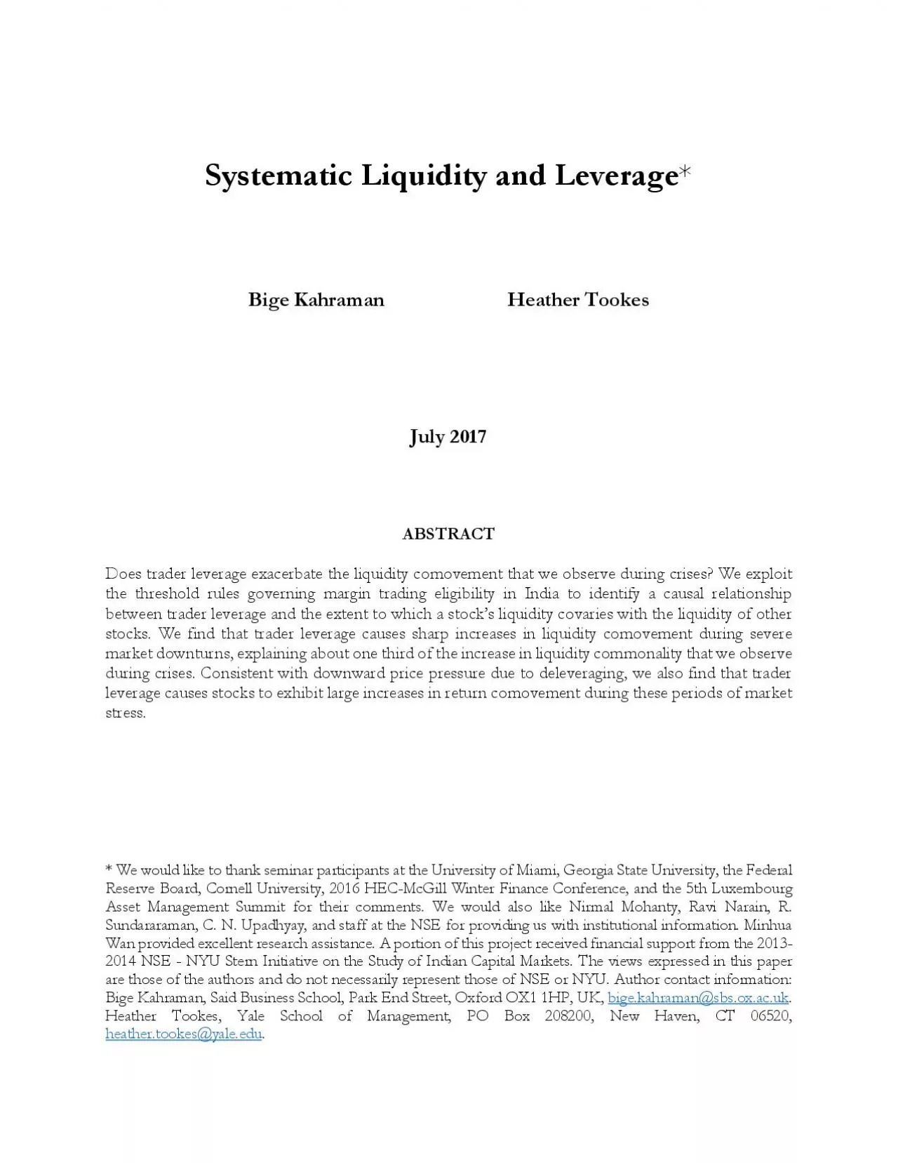
Heather Tookes Yale School of Management PO Box 208200 New Haven CT 06520 heathertookesyaleeduDoes trader leverage exacerbate the liquidity comovement that we observe

Presentation Embed Code

<iframe width="560" height="315" src="https://www.docslides.com/embed/871282" frameborder="0" allowfullscreen></iframe>

Download Presentation

Download Presentation The PPT/PDF document "Does trader leverage exacerbate the liqu..." is the property of its rightful owner. Permission is granted to download and print the materials on this website for personal, non-commercial use only, and to display it on your personal computer provided you do not modify the materials and that you retain all copyright notices contained in the materials. By downloading content from our website, you accept the terms of this agreement.

Does trader leverage exacerbate the liquidity comovement that we obser: Transcript

Download Document

Here is the link to download the presentation.
"Does trader leverage exacerbate the liquidity comovement that we obser"The content belongs to its owner. You may download and print it for personal use, without modification, and keep all copyright notices. By downloading, you agree to these terms.