RF Communication Circuits

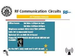
Office hours Sat Mon 130pm to 2pm Sat Mon 600pm 630pm Telephone contact 09121117364 RFMi Calls OK in reasonable hours Technical Qs on SMS OK 24 hours Please DO NOT KNOCK ON MY DOOR BEFORE MY CLASSES

Embed this Presentation

Download Notice

Download Presentation The PPT/PDF document "RF Communication Circuits" is the property of its rightful owner. Permission is granted to download and print the materials on this website for personal, non-commercial use only, and to display it on your personal computer provided you do not modify the materials and that you retain all copyright notices contained in the materials. By downloading content from our website, you accept the terms of this agreement.