/
Ph/CS 219A Quantum Computation Lecture 6. Bell Inequalities Ph/CS 219A Quantum Computation Lecture 6. Bell Inequalities

Ph/CS 219A Quantum Computation Lecture 6. Bell Inequalities - PowerPoint Presentation

emmy
emmy . @emmy
Follow
342 views
Uploaded On 2022-05-31

Ph/CS 219A Quantum Computation Lecture 6. Bell Inequalities - PPT Presentation

1 Ph CS 219A Quantum Computation Lecture 6 Bell Inequalities Today we start a new topic We will explore more deeply how quantum correlations are different from classical ones Two parties in different laboratories who share quantum entanglement but are unable to communicate can perform ID: 912428

alice bob waterloo coins bob alice coins waterloo pasadena donald coin tails heads bell probability uncover outcomes quantum correlated

Share:

Link:

Embed:

Download Presentation from below link

Download Presentation The PPT/PDF document "Ph/CS 219A Quantum Computation Lecture 6..." is the property of its rightful owner. Permission is granted to download and print the materials on this web site for personal, non-commercial use only, and to display it on your personal computer provided you do not modify the materials and that you retain all copyright notices contained in the materials. By downloading content from our website, you accept the terms of this agreement.


Presentation Transcript

Slide1

Ph/CS 219A Quantum Computation Lecture 6. Bell Inequalities

1

Ph/CS 219AQuantum Computation

Lecture

6. Bell Inequalities

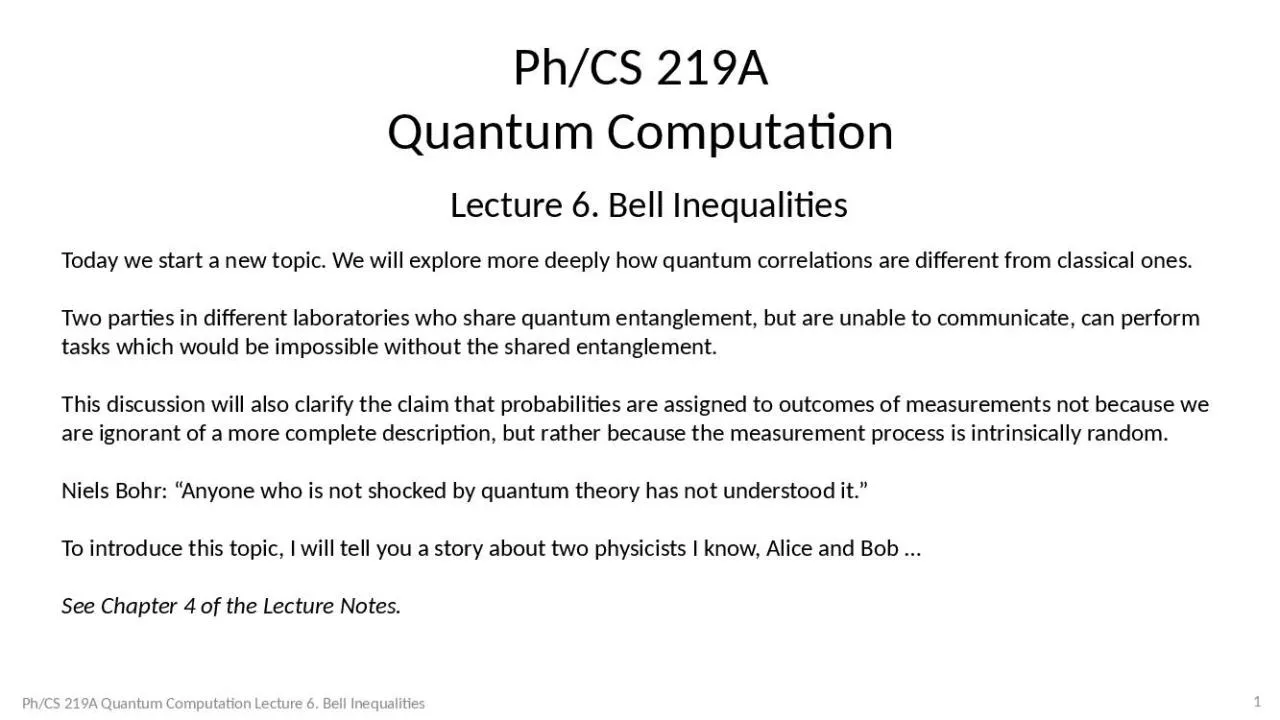
Today we start a new topic. We will explore more deeply how quantum correlations are different from classical ones.

Two parties in different laboratories who share quantum entanglement, but are unable to communicate, can perform tasks which would be impossible without the shared entanglement.

This discussion will also clarify the claim that probabilities are assigned to outcomes of measurements not because we are ignorant of a more complete description, but rather because the measurement process is intrinsically random.

Niels Bohr: “Anyone who is not shocked by quantum theory has not understood it.”

To introduce this topic, I will tell you a story about two physicists I know, Alice and Bob …

See Chapter

4

of the Lecture Notes.

Slide2

Three coins on the table. Each is either heads or tails. You can uncover any one of the three coins, revealing whether it is heads of tails, but when you two the other two coins disappear --- you’ll never know whether those other two coins are heads or tails.

1

2

3

Slide3

Three coins on the table. Each is either heads or tails. You can uncover any one of the three coins, revealing whether it is heads of tails, but when you two the other two coins disappear --- you’ll never know whether those other two coins are heads or tails.

1

2

3

Slide4

Three coins on the table. Each is either heads or tails. You can uncover any one of the three coins, revealing whether it is heads of tails, but when you two the other two coins disappear --- you’ll never know whether those other two coins are heads or tails.

1

2

3

Slide5

Three coins on the table. Each is either heads or tails. You can uncover any one of the three coins, revealing whether it is heads of tails, but when you two the other two coins disappear --- you’ll never know whether those other two coins are heads or tails.

1

2

3

Slide6

Alice (Pasadena)

Bob (Waterloo)

Donald

(Denver)

There are many sets of coins, identically prepared by Donald.

For each of the three coins, in Pasadena or Waterloo, the probability is ½ that the coin is heads or tails.

1

2

3

1

2

3

Slide7

Alice (Pasadena)

Bob (Waterloo)

There are many sets of coins, identically prepared by Donald.

For each of the three coins, in Pasadena or Waterloo, the probability is ½ that the coin is heads or tails.

But, if Alice and Bob both uncover the same coin, the outcomes are perfectly correlated.

Donald

(Denver)

1

2

3

1

2

3

Slide8

Alice (Pasadena)

Bob (Waterloo)

There are many sets of coins, identically prepared by Donald.

For each of the three coins, in Pasadena or Waterloo, the probability is ½ that the coin is heads or tails.

But, if Alice and Bob both uncover the same coin, the outcomes are perfectly correlated.

Donald

(Denver)

1

2

3

1

2

3

Slide9

Alice (Pasadena)

Bob (Waterloo)

There are many sets of coins, identically prepared by Donald.

For each of the three coins, in Pasadena or Waterloo, the probability is ½ that the coin is heads or tails.

But, if Alice and Bob both uncover the same coin, the outcomes are perfectly correlated.

Donald

(Denver)

1

2

3

1

2

3

Slide10

Alice (Pasadena)

Bob (Waterloo)

There are many sets of coins, identically prepared by Donald.

For each of the three coins, in Pasadena or Waterloo, the probability is ½ that the coin is heads or tails.

But, if Alice and Bob both uncover the same coin, the outcomes are perfectly correlated.

Donald

(Denver)

1

2

3

1

2

3

Slide11

Alice (Pasadena)

Bob (Waterloo)

Donald

(Denver)

1

2

3

1

2

3

There are many sets of coins, identically prepared by Donald.

For each of the three coins, in Pasadena or Waterloo, the probability is ½ that the coin is heads or tails.

But, if Alice and Bob both uncover the same coin, the outcomes are perfectly correlated.

We know it always works – we’ve checked it a million times.

Slide12

Alice (Pasadena)

Bob (Waterloo)

There are many sets of coins, identically prepared by Donald.

For each of the three coins, in Pasadena or Waterloo, the probability is ½ that the coin is heads or tails.

But, if Alice and Bob both uncover the same coin, the outcomes are perfectly correlated.

We know it always works – we’ve checked it a million times.

Donald

(Denver)

1

2

3

1

2

3

Slide13

Alice (Pasadena)

Bob (Waterloo)

Donald

(Denver)

1

2

3

1

2

3

There are many sets of coins, identically prepared by Donald.

For each of the three coins, in Pasadena or Waterloo, the probability is ½ that the coin is heads or tails.

But, if Alice and Bob both uncover the same coin, the outcomes are perfectly correlated.

We know it always works – we’ve checked it a million times.

Slide14

Alice (Pasadena)

Bob (Waterloo)

There are many sets of coins, identically prepared by Donald.

For each of the three coins, in Pasadena or Waterloo, the probability is ½ that the coin is heads or tails.

But, if Alice and Bob both uncover the same coin, the outcomes are perfectly correlated.

We know it always works – we’ve checked it a million times.

Donald

(Denver)

1

2

3

1

2

3

Slide15

Alice (Pasadena)

Bob (Waterloo)

Donald

(Denver)

1

2

3

1

2

3

There are many sets of coins, identically prepared by Donald.

For each of the three coins, in Pasadena or Waterloo, the probability is ½ that the coin is heads or tails.

But, if Alice and Bob both uncover the same coin, the outcomes are perfectly correlated.

We know it always works – we’ve checked it a million times.

Slide16

Alice (Pasadena)

Bob (Waterloo)

Donald

(Denver)

1

2

3

1

2

3

Bob reasons:

-- We know the correlation is always perfect,

-- And surely what Alice does in Pasadena exerts no influence on what Bob finds when he uncovers a coin in Waterloo.

-- So, in effect, Alice and Bob, working together, can learn the outcome when any two of the coins are uncovered in Waterloo.

Slide17

Alice (Pasadena)

Bob (Waterloo)

Donald

(Denver)

1

2

3

1

2

3

Bob reasons:

-- We know the correlation is always perfect,

-- And surely what Alice does in Pasadena exerts no influence on what Bob finds when he uncovers a coin in Waterloo.

-- So, in effect, Alice and Bob, working together, can learn the outcome when any two of the coins are uncovered in Waterloo.

Slide18

Alice (Pasadena)

Bob (Waterloo)

Donald

(Denver)

1

2

3

1

2

3

Bob reasons:

-- We know the correlation is always perfect,

-- And surely what Alice does in Pasadena exerts no influence on what Bob finds when he uncovers a coin in Waterloo.

-- So, in effect, Alice and Bob, working together, can learn the outcome when any two of the coins are uncovered in Waterloo.

Slide19

Alice (Pasadena)

Bob (Waterloo)

Donald

(Denver)

1

2

3

1

2

3

Bob reasons:

-- We know the correlation is always perfect,

-- And surely what Alice does in Pasadena exerts no influence on what Bob finds when he uncovers a coin in Waterloo.

-- So, in effect, Alice and Bob, working together, can learn the outcome when any two of the coins are uncovered in Waterloo.

Slide20

Alice (Pasadena)

Bob (Waterloo)

Bell reasons:

Why? Because if you uncover all three coins, at least two have to be the same!

Slide21

Alice (Pasadena)

Bob (Waterloo)

Alice and Bob did the experiment a million times, and found …

How could Bell’s prediction be wrong? Bell assumed the probability distribution describes our ignorance about the actually state of the coins under the black covers, and that there is no “action at a distance” between Pasadena and Waterloo. The lesson:

-- Don’t reason about “counterfactuals” (“I found H when I uncovered 1; I would have found either H or T if I had uncovered 2 instead, I just don’t know which.”) When the measurements are incompatible, then if we do measurement 1 we can’t speak about what would have happened if we had done measurement 2 instead.

-- Quantum randomness is not due to ignorance. Rather, it is intrinsic, occurring even when we have the most complete knowledge that Nature will allow.

-- Note that the quantum correlations do not allow A and B to send signals to one another.

Slide22

Alice (Pasadena)

However, Alice and Bob did the experiment a million times, and found …

Bell inequality violations are seen in experiments with qubits encoded in photons, atoms,

electron spins, and

superconducting circuits.

There are “loopholes”:

Detection efficiency

Causality

“Free will”

Bell inequality violation has been verified experimentally since the 1980s, but the first “loophole free” experiments were achieved in 2015.

Alice and Bob shared a maximally entangled (Bell) pair of qubits, and each could perform a two-outcome measurement on her/his qubit in one of three possible ways. What did they measure?

Bob

(Waterloo)

Slide23

Ph/CS 219A Quantum Computation Lecture 6. Bell Inequalities

23

Okay, what’s

really

going on?

Donald

prepares a maximally entangled state of two qubits:

For Alice, the three coins that

can be uncovered are three possible single-qubit observables that she may choose to measure, and same for Bob. These three operators are

noncommuting

, so measuring one disturbs a measurement of the others. That is why when Alice uncovers a coin (measures one of the observables), the other coins disappear (she can’t know what would have happened if she had measured these observables instead).

Heads and tails are two possible outcomes of measuring an observable which has eigenvalues +1 and -1. Because the state prepared by Donald is

entangled,

Alice’s measurement outcomes are correlated with Bob’s. The observables they measure have the form.

You can check:

Therefore:

(repeated indices summed)

Slide24

Ph/CS 219A Quantum Computation Lecture 6. Bell Inequalities

24

Okay, what’s

really

going on?

When Alice and Bob “uncover

the same coin” their measurement axes are

anti-aligned

. Then they always get the same measurement outcome.

When Alice and Bob “uncover different coins” the angle between their measurement axes is 60 degrees. In that case they get the same measurement outcome with probability ¼.

Bell was wrong, because he assumed incorrectly that he could assign probabilities of outcomes to measurements that were not performed.

The randomness of the outcomes is not due to ignorance --- it is

intrinsic

.

Slide25

Ph/CS 219A Quantum Computation Lecture 6. Bell Inequalities

25

Clauser

-Horne-

Shimony

-Holt

(CHSH) Inequality

Suppose the randomness

of the outcomes is due to ignorance. If we had complete information we would know with certainty the values of:

A

B

bits

a

,a

1

1

b,b

correlated

Notice that:

Consider:

This is the CHSH Inequality.

(

Clauser

was a Caltech physics BA, 1964.)

For a joint probability distribution governing these four binary

variables:

Slide26

Ph/CS 219A Quantum Computation Lecture 6. Bell Inequalities

26

Clauser

-Horne-

Shimony

-Holt

(CHSH) Inequality

A

B

bits

a

,a

1

1

b,b

correlated

The CHSH inequality

is violated.

Slide27

Ph/CS 219A Quantum Computation Lecture 6. Bell Inequalities

27

Clauser

-Horne-

Shimony

-Holt

(CHSH) Inequality

This the choice

of binary observables that

maximally

violates the CHSH inequality.

(

Cirel’son

Inequality)

Slide28

Ph/CS 219A Quantum Computation Lecture 6. Bell Inequalities

28

Clauser

-Horne-

Shimony

-Holt

(CHSH) Inequality

Bell inequality violations are seen in experiments with qubits encoded in photons, atoms,

electron spins, and

superconducting circuits.

There are “loopholes”:

Detection

efficiency. Alice and Bob don’t have a fair sample because detection sometimes fails.

Causality. E.g., A measures first, and by the time B measures, a signal could have traveled A

 B.

“Free will

”. Hidden variables govern not only the outcomes, but also what A and B “choose” to measure.

Bell inequality violation has been verified experimentally since the 1980s, but the first “loophole free” experiments were achieved in 2015

. These simultaneously close the detection and causality loopholes.

Bell inequality violations have been seen in experiments where A and B measurement choices of what to measure are governed by brightness fluctuations in stars hundreds of light years apart.

Slide29

Ph/CS 219A Quantum Computation Lecture 6. Bell Inequalities

29

CHSH Game

CHSH inequality:

A

B

bits

a

y

x

b

Goal:

correlated

Averaged uniformly over inputs, no “classical strategy” can win the game with success probability better than .75

For “quantum strategies”, the highest possible success probability improves to

Slide30

Ph/CS 219A Quantum Computation Lecture 6. Bell Inequalities

30

Bell inequalities more

g

enerally

Now

a, b

are possible measurement “settings” for Alice and Bob, taking

m

possible values.

And

x, y

are possible measurement “outcomes” taking

v

possible values.

A

B

bits

a

y

x

b

correlated

In a “local configuration” there is a definite

x

for each

a

(

which does not depend on

b

)

, and a definite

y

for each

b

(which does not depend on

a

).

A “local model” also known as a “local hidden variable theory” (LHVT) assigns a probability to each local configuration.

Bell inequalities

are constraints on

p(

xy|ab

)

that apply to any local model.