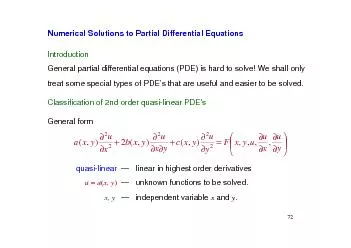
74GeometricallyType may not be constant over R because abc can vary - PDF document

1 74GeometricallyType may not be constant
74GeometricallyType may not be constant over R because a,b,c can vary over R, e.g, elliptic in one part of Rand parabolic in the other part of R.Example: ellipticparabolic Rîí=£-=-Þ===Þ££-££-+-=+000sin1,0,sin33,33:])(sin[)(sin2222yacbcbyayxuyuuuayxyyxx43421 R 75General Approach to the Solutions of PDEsStep 1: Define a grid on Rwith “me

2 sh points” k jR hi xy mesh point pi
sh points” k jR hi xy mesh point pij=(ih, jk) Step 2: Approximate derivatives at mesh points by central difference quotients 21,,1,2,1,,11,1,,1,12),(,2),(,2),(,2),(kuuujkihuhuuujkihukuujkihuhuujkihujijijiyyjijijixxjijiyjijix-+-+-+-++-=+-=-=-=These will bring a PDE to a difference equation relating uijto its neighbouringpoints in the grid. 76For example,

3 022021,,1,2,1,,1=+-++-Þ=+-+-+kuuuhuuuuu
022021,,1,2,1,,1=+-++-Þ=+-+-+kuuuhuuuuujijijijijijiyyxx0)(2,221,21,2,12,12=+-+++-+-+jijijijijiuhkuhuhukuk Step 3: Arrange the resulting difference equation into a system of linear equationsúúúûùêêêëé=úúúûùêêêëéúúúûùêêêëé*************1211MMLMOMMLuu,...,1211uu Taking into consideration of boundary conditions and solve it for Step

4 4: change grid size for a more accurate
4: change grid size for a more accurate approximation. LLLL4242kkkhhh®®®®n 77Solution to Elliptic Type’s PDEThe general approach will be followed to solve these types of problems by taking into account various kinds of boundary conditions in formof the system of linear equations. We will illustrate this using the following PDE: 0),(2222º=+=¶¶+Â

5 ¶yxfuuyuxuyyxx)1(log)1(),(10xyyxu++= c
¶yxfuuyuxuyyxx)1(log)1(),(10xyyxu++= condition Boundary{}30,30),,(££££=yxyxRWe follow the step-by-step procedure given in the previous section. 78Step 1:Define a grid along with an order of mesh-points inside R. (We have to be clear about Rand h, k )First, let us start with a crude grid h = k = 3/N, forN=3—� h = k = 1 11u21u31u01u20u10u32u2

6 2u12u02u13u23u0123123 )1(log410xu+= 4log
2u12u02u13u23u0123123 )1(log410xu+= 4log)1(10yu+= )1(log10xu+= 0=uknowns: 2010010231322313,,,,,,,uuuuuuuuunknowns: 22211211,,,uuuu 79Step 2:Approximate derivatives at mesh-pointsAt mesh-point (i, j)where is unknown: 043,2,13,2,10220),(,1,1,,1,121,,1,2,1,,1=-+++Þ==º=+-++-Þ==+-+-+-+-+jijijijijiijjijijijijijiyyxxuuuuujifkuuuhuuuyxfuujiu, 121021011112

7 11102111014220uuuuuuuuuuu++++-=+-++-=212
11102111014220uuuuuuuuuuu++++-=+-++-=212220311140uuuuu-+++=@ (1,1): 00.301@ (2,1): 1.2040.477@ (1,2):122202131140uuuuu-+++= 1.2040@ (2,2):223212232140uuuuu-+++= 1.9081.806 Boundary valuesare known 80Step 3:Arrange the equation into matrix formSolve the equations forStep 4:Refine the step-size by choosing smaller h, k.÷÷÷÷÷øöçççççèæ----=÷÷÷÷Ã

8 ·Ã¸Ã¶Ã§Ã§Ã§Ã§Ã§Ã¨Ã¦Ã·Ã·Ã·Ã·Ã·Ã¸Ã¶Ã§Ã§Ã§Ã
·Ã¸Ã¶Ã§Ã§Ã§Ã§Ã§Ã¨Ã¦Ã·Ã·Ã·Ã·Ã·Ã¸Ã¶Ã§Ã§Ã§Ã§Ã§Ã¨Ã¦----681.1301.0714.3204.14110140110410114211112uuu÷÷÷÷øöççççèæ=÷÷÷÷÷øöçççççèæ875.0483.0336.1756.021112212uuuu 81Parabolic and Hyperbolic TypesParabolic: Example —heat equationHyperbolic:Example —wave equationWe will use parabolic type to illustrate the solution

9 method, which carries over to the hyperb
method, which carries over to the hyperbolic type as well!tcoefficien diffusion heat is whereDuDutxx,=ttxxuuC=2txxuu=where C 2is wave propagation velocity R0=xLx= h k Boundary condition:u(L, t) =uL(t) Boundary condition:u(0, t) =u0(t) initial conditiont 82Notations:ThenTo solve the equation, we start with j = 0, then ’s are given as initial cond

10 itions and can be used to solve for 2,1
itions and can be used to solve for 2,1,,1211,1,1,2),(),(2),(),(),(),(),(),(,1,0,,,,1,0,huuuhtxutxutxutxukuuktxutxutxutxuujkjtNLhNhLNihixjijijijijijijixxjijijijijitjijiji-+-++++-=+-=-=-===×==Þ==×=LL ()jii,j,jii,ji,jxxtuuu h kDuu D uu,11212-+++-=-Þ=0,iu1,,1,1,-=NiuiL (§)Prepared by Ben M. Chen 83Rewrite equation (§) as() 2,111with 21hkDuuu

11 ujii,j,jii,j=×+-+×=-++ggggIn general,
ujii,j,jii,j=×+-+×=-++ggggIn general, we can solve for ui,j+1,i= 1, ¼, N,if we know the j-th row. 011-NNj1+j0,1u0,1-Nuju,1jNu,1-1,1+-jNu1,1+ju boundarycondition boundarycondition initial condition 84Example:Solve the following boundary value problem,We choose N = 3and hence h= 1/3 and choose two different k:1,1,10,==££=LDxuuxxt 2sin)0,(xxup=initial condi

12 tion:1),1(,0),0(==tutu boundary conditi
tion:1),1(,0),0(==tutu boundary condition:45.005.0==gak9.01.0==gak ijkju,0ju,1ju,2ju,3 ju,1ju,2 ijk866.0500.00.01866.0500.0000.0657.0379.01.01762.0434.0005.0716.0288.02.01724.0387.0010.0587.0414.03.01696.0364.0015.0803.0197.04.01684.0350.0020.0435.0505.05.01676.0343.0025.0061.1061.06.01672.0338.0030.0-003.0003.17.01667.0336.0035.0-805.1804.08.01668.0335.0040

13 .0-269.1269.29.01668.0334.0045.0-457.395
.0-269.1269.29.01668.0334.0045.0-457.3957.20.11667.0333.0050.0- unstablecase 85A short discussion about hyperbolic type PDE:0,10,),(2³££=txutxCuxxtt Initial conditions:)()0,(),()0,(21xfxuxfxut==PDE:Boundary conditions:)(),1(),(),0(10tgtutgtu==() 222*1,,1*,1**122 h kCuuuuujijijii,ji,j=-×+×+-=-+-+gggg withFollowing the usual procedure, we obtain an app

14 roximation:Note that atj = 0, we have to
roximation:Note that atj = 0, we have to deal with , which are not readily available.Thus, we will have to compute these terms first.1,-iu)(2)(2)()0,(21,1,21,1,2iiiiiitxkfuuxkfuuxfxu-=Þ=-Þ=-- 86The difference equation can then be solved by using the direct method, e.g,)(2***)22(**)22(21,0,10,10,1,0,1*0,10,1,iiiiiiiiiixkfuuuuuuuuu+-++-=-++-=+--+-gggg

15 gg 1,,2,1),()(*21)(*2)(*)1(2111111,-=+++
gg 1,,2,1),()(*21)(*2)(*)1(2111111,-=+++-=+-NixkfxfxfxfuiiiiiLggg For j� 1, we still use()1,,1*,1**122-+-+-×+×+-=jijijii,ji,juuuuuggg The rest of computational procedure is exactly the same as that in the parabolic case.n 87Example:SolveLet us choose h= k= 0.25so that g* = 1Determine to start the solution or use formula on the previous paget

16 o compute , i = 1, 2, 3,first, i.e
o compute , i = 1, 2, 3,first, i.e.,()()()()()()()()() ()ttgtutgtuconditionsBoundaryxxxfxuxfxuconditionsInitialtxuuPDEtxxttpppsin1,10,0sin0,00,:0,10:1021====+====³££= : 1,iu1,-iu[]ïîïíì===Þ+=×+=364.0375.0239.0)sin(25.0)(01,31,21,121,uuuðxxxfkuiiiiD.I.Y. to complete the solutions up to