PDF-How to interpret results of meta

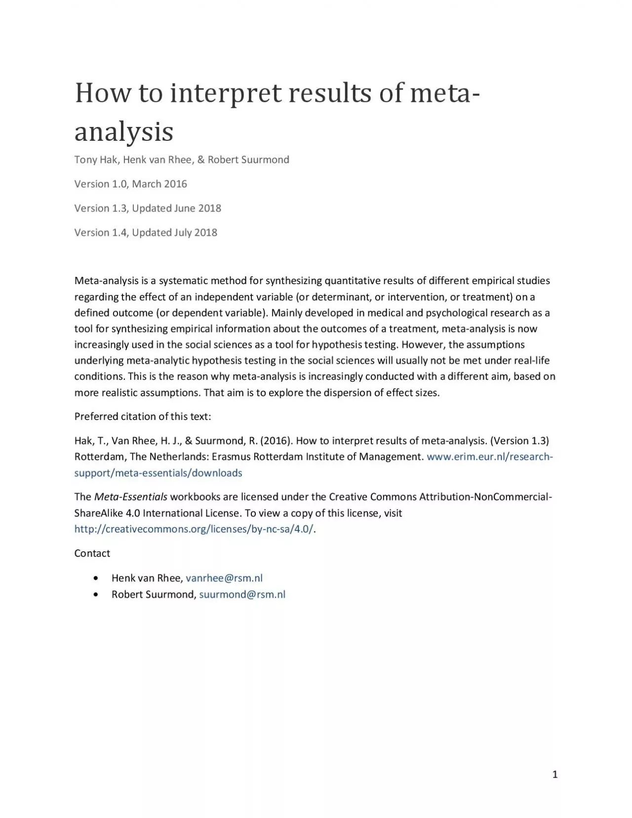
1 analysis Tony Hak Henk van Rhee Robert Suurmond Version 10 March 2016 Version 13 Updated June 2018 Version 1 4 Updated July 2018 Meta analysis is a systematic method for synthesizing. interpret the results of individual studies in the context of other research that has been done. This is especially important for decisions about whether a medical treatment works and for deci si PDF4LHC combinations. . Jun Gao, Joey Huston, . Pavel Nadolsky (presenter). arXiv:1401.0013, http. ://metapdf.hepforge.org. Parton distributions for the LHC, . Benasque. , 2019-02-19, 2015. A . meta-analysis . and SCD Meta-Analyses. William R. Shadish. University of California, Merced. Borrowing liberally from coauthored work with Larry Hedges, David . Rindskopf. , James . Pustejovsky. , . Kristynn. Sullivan, Jonathan . de chimiothérapie dans les cancers des . VADS: actualisation. Jean-Pierre . Pignon. , . Pierre . Blanchard, . Anne . Lee, . Laureen. . Majed. , Sophie . Marguet. , . Claire . Petit, Cécile . Landais. Professor, Stanford University; . Director. , Stanford Prevention Research Center . Evidence-based medicine has been hijacked. Lown Conference, Chicago, 4/2016. John P.A. Ioannidis, MD, DSc. C.F. Rehnborg Chair in Disease Prevention. Teleconference . November 21, . 2016. 2. PM GMT (Greenwich . Mean. Time). Amsterdam/Barcelona/Berlin/Milan/Munich/Rome/Zurich 3 PM. Oxford/Braga 2 PM. Sao Paulo . noon. Tokyo/Kyoto/Seoul 11 PM. Cape Town 4 PM. Sven . Kepes & Michael A. McDaniel. April 29, 2017. Outline. Meta-analysis . and cumulative knowledge . Sensitivity analysis. Sensitivity analysis: . Outliers. Sensitivity analysis: Publication . Publication Bias: Causes, Detection, and Remediation Sven Kepes and Michael A. McDaniel Virginia Commonwealth University AOM PDW August 2, 2014 Philadelphia, PA   http://tinyurl.com/nfayr3r Overview 5x improvement . in system development speed over current . practice. In order to. do this metrics need to be used to synthesize and select the best possible system architecture:. A key element is to choose system architectures and designs that achieve desired performance . Jaswin Sawhney. Maine Medical Center. Portland, Maine. Introduction to Meta-Analysis. What is a systematic review? . A systematic review is a research methodology that tries to identify, select, appraise, and synthesize all research evidence relevant to a specific research question . Hardy-Weinberg equilibrium. Meta-analysis. SNP Imputation. Review what we have learned about the genetics of common disease from GWAS. Where do we go from here? What do we go with GWAS results.. functional characterization of GWAS loci. Objective. Understand the philosophy of meta-analysis and its contribution to epidemiology and science.. Understand the limitations of meta-analysis. Introduction. Systematic quantitative integration of results . highly active antiretroviral . therapy (HAART). As PLHIV age, they also develop other co-morbidities like obesity, diabetes, and cardiovascular diseases. . In this study, we reviewed published literature on . Presented by Christine R. Wells, Ph.D.. Statistical Methods and Data Analytics. UCLA Office of Advanced Research Computing. What to expect from this workshop. Definition of systematic review and meta-analysis.