/
Hardy Weinberg Equilibrium Hardy Weinberg Equilibrium

Hardy Weinberg Equilibrium - PowerPoint Presentation

ginocrossed
ginocrossed . @ginocrossed
Follow
345 views
Uploaded On 2020-06-16

Hardy Weinberg Equilibrium - PPT Presentation

Wilhem Weinberg 1862 1937 Gregor Mendel G H Hardy 1877 1947 18221884 Lectures 411 Mechanisms of Evolution Microevolution Hardy Weinberg Principle Mendelian Inheritance ID: 778718

population allele weinberg generation allele population generation weinberg hardy equilibrium frequencies alleles genotype frequency recessive selection dominant expected deviation

Share:

Link:

Embed:

Download Presentation from below link

Download The PPT/PDF document "Hardy Weinberg Equilibrium" is the property of its rightful owner. Permission is granted to download and print the materials on this web site for personal, non-commercial use only, and to display it on your personal computer provided you do not modify the materials and that you retain all copyright notices contained in the materials. By downloading content from our website, you accept the terms of this agreement.


Presentation Transcript

Slide1

Hardy Weinberg Equilibrium

Wilhem Weinberg

(1862 – 1937)

Gregor Mendel

G. H. Hardy

(1877 - 1947)

(1822-1884)

Slide2

Lectures 4-11: Mechanisms of Evolution (Microevolution)

Hardy Weinberg Principle (Mendelian

Inheritance)Genetic DriftMutationSex: Recombination and Random Mating

Epigenetic InheritanceNatural SelectionThese are mechanisms acting WITHIN populations, hence called “population genetics”—EXCEPT for epigenetic modifications, which act on individuals in a Lamarckian manner

Slide3

Evolution acts through

changes in allele frequency at each generation

Leads to

average change in characteristic of the population

Recall from Previous Lectures

Darwin’s Observation

Slide4

HOWEVER, Darwin did not understand how genetic variation was passed on from generation to generation

Recall from Lecture on History of Evolutionary Thought

Darwin

s Observation

Slide5

Gregor Mendel,

“Father of Modern Genetics

Mendel presented a mechanism for how traits got passed on

Individuals pass alleles on to their offspring intact”

(the idea of particulate (genes) inheritance)

Gregor Mendel

(1822-1884)

http://www.biography.com/people/gregor-mendel-39282#synopsis

Slide6

Gregor Mendel,

“Father of Modern Genetics

Mendel’

s Laws of InheritanceLaw of Segregationonly one allele passes from each parent on to an offspringLaw of Independent Assortment

different pairs of alleles are passed to offspring independently of each other

Gregor Mendel

(1822-1884)

http://www.biography.com/people/gregor-mendel-39282#synopsis

Slide7

Gregor Mendel

Slide8

In cross-pollinating plants with either yellow or green peas, Mendel found that the first generation (f1) always had yellow seeds (dominance).   However, the following generation (f2) consistently had a 3:1 ratio of yellow to green.

Using 29,000 pea plants, Mendel discovered the 1:3 ratio of phenotypes, due to dominant

vs.

recessive alleles

Slide9

Mendel uncovered the underlying mechanism, that there are dominant and recessive alleles

Slide10

Mathematical description of

Mendelian inheritance

Hardy-Weinberg Principle

Godfrey Hardy

(1877-1947)

Wilhem

Weinberg

(1862 – 1937)

Slide11

Testing for Hardy-Weinberg equilibrium can be used to assess whether a population is evolving

Slide12

The Hardy-Weinberg Principle

A population that is not evolving shows allele and genotypic frequencies that are in

Hardy Weinberg equilibriumIf a population is not in Hardy-Weinberg equilibrium, it can be concluded that the population is evolving

Slide13

Evolutionary Mechanisms

(will put population out of HW Equilibrium):

Genetic Drift

Natural Selection

Mutation

Migration

*

Epigenetic modifications

change expression of alleles but not the frequency of alleles themselves, so they won’t affect the actual inheritance of alleles

However, if you count the

phenotype frequencies,

and not the

genotype frequencies

, you might see phenotypic frequencies out of HW Equilibrium due to epigenetic silencing of alleles. (epigenetic modifications can change phenotype, not genotype

)

Slide14

Requirements of HW

Evolution

Large population size

Genetic drift

Random Mating

Inbreeding & other

No Mutations

Mutations

No Natural Selection

Natural Selection

No Migration

Migration

An evolving population is one that violates Hardy-Weinberg Assumptions

Violation

Slide15

Fig. 23-5a

Porcupine

herd range

Beaufort Sea

NORTHWEST

TERRITORIES

MAP

AREA

ALASKA

CANADA

Fortymile

herd range

ALASKA

YUKON

What is a “

population

?”

A group of individuals within a species that is capable of interbreeding and producing fertile offspring

(definition for sexual species)

Slide16

Patterns of inheritance should always be in “Hardy Weinberg Equilibrium”

Following the transmission rules of Mendel

In the absence of Evolution…

Slide17

Hardy-Weinberg Equilibrium

According to the

Hardy-Weinberg principle,

frequencies of alleles and genotypes

in a population remain constant from generation to generation

Also, the genotype frequencies you see in a population should be the Hardy-Weinberg expectations, given the allele frequencies

Slide18

“Null Model”

No Evolution: Null Model to test if no evolution is happening should simply be a population in Hardy-Weinberg EquilibriumNo Selection:

Null Model to test whether Natural Selection is occurring should have no selection, but should include Genetic DriftThis is because Genetic Drift is operating even when there is no Natural Selection

Slide19

Example

: Is this population in Hardy Weinberg Equilibrium?

AA Aa

aa Generation 1

0.25 0.50 0.25

Generation 2 0.20 0.60 0.20

Generation 3

0.10 0.80 0.10

Slide20

Hardy-Weinberg Theorem

In a non-evolving population, frequency of alleles and genotypes remain

constant

over generations

You should be able to predict the genotype frequencies, given the allele frequencies

Slide21

important concepts

gene: A region of genome sequence (DNA or RNA), that is the unit of inheritance , the product of which contributes to phenotypelocus

: Location in a genome (used interchangeably with “gene,” if the location is at a gene… but, locus can be anywhere, so meaning is broader than gene)loci

: Plural of locusallele: Variant forms of a gene (e.g. alleles for different eye colors, BRCA1 breast cancer allele, etc.)genotype: The combination of alleles at a locus (gene)

phenotype: The expression of a trait, as a result of the genotype and regulation of genes (green eyes, brown hair, body size, finger length, cystic fibrosis, etc.)

Slide22

important concepts

allele: Variant forms of a gene (e.g. alleles for different eye colors, BRCA1 breast cancer allele, etc.)

We are diploid (2 chromosomes), so we have 2 alleles at a locus (any location in the genome)

However, there can be many alleles at a locus in a population.For example, you might have inherited a blue eye allele from your mom and a brown eye allele from your dad… you can’t have more alleles than that (only 2 chromosomes, one from each parent)BUT, there could be many alleles at this locus in the population, blue, green, grey, brown, etc.

Slide23

Alleles

in a population of diploid organisms

A1

A2

A3

A4

A1

A1

A2

Sperm

Eggs

Genotypes

Random Mating (Sex)

Zygotes

A1A3

A1A1

A1A1

A2A4

A3A1

A1A1

A1

A2

A1

A1

A3

A4

Slide24

So then can we predict the % of alleles and genotypes in the population at each generation?

A1

A2

A3

A4

A1

A1

A2

Sperm

Eggs

Zygotes

A1A3

A1A1

A1A1

A2A4

A3A1

A1A1

A1

A2

A1

A1

A3

A4

Slide25

Hardy-Weinberg Theorem

In a non-evolving population, frequency of alleles and genotypes remain

constant

over generations

Slide26

Fig. 23-6

Frequencies of alleles

Alleles in the population

Gametes produced

Each egg:

Each sperm:

80%

chance

80%

chance

20%

chance

20%

chance

q

= frequency of

p

= frequency of

C

R

allele = 0.8

C

W

allele = 0.2

Hardy-Weinberg proportions indicate the expected allele and genotype frequencies, given the starting frequencies

Slide27

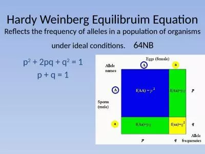
By convention, if there are 2 alleles at a locus, p and q are used to represent their frequencies

The frequency of all alleles in a population will add up to 1For example, p

+ q = 1

Slide28

If p and

q represent the relative frequencies of the only two possible alleles in a population at a particular locus, then for a diploid organism (2 chromosomes),

(p +

q) 2 = 1 = p

2 + 2pq + q2 = 1

where p2

and q2 represent the frequencies of the homozygous genotypes and 2pq represents the frequency of the heterozygous genotype

Slide29

What about for a triploid organism?

Slide30

What about for a triploid organism?

(p +

q)3 = 1

= p3 + 3p

2q + 3pq2

+ q3 = 1

Potential offspring: ppp,

ppq

,

pqp

,

qpp

,

qqp

,

pqq

,

qpq

,

qqq

How about

tetraploid? You work it out.

Slide31

Hardy Weinberg Theorem

ALLELES

Probability of

A

= p p

+ q

= 1Probability of

a

=

q

GENOTYPES

AA

:

p

x

p

=

p2Aa: p x q + q

x

p

= 2

p

q

aa

:

q

x

q

=

q

2

p

2

+ 2

p

q

+

q

2

= 1

Slide32

More General HW Equations

One locus three alleles: (p + q + r)

2 = p2 + q2 + r

2 + 2pq +2pr + 2qrOne locus n # alleles: (p1 + p2 + p3 + p4

… …+ pn)2 = p12 + p22 + p

32 + p42… …+ p

n2 + 2p1p2 + 2p1p

3

+ 2p

2

p

3

+ 2p

1

p

4

+ 2p

1

p

5

+ … … + 2pn-1pnFor a polyploid (more than two chromosomes):

(p + q)c, where c = number of chromosomesIf multiple loci (genes) code for a trait, each locus follows the HW principle independently, and then the alleles at each loci interact to influence the trait

Slide33

ALLELE Frequencies

Frequency of A =

p

= 0.8

Frequency of a =

q

= 0.2

p

+

q

= 1

Expected GENOTYPE Frequencies

AA:

p

x

p

= p

2

= 0.8

x

0.8 = 0.64

Aa

:

p

x

q

+

q

x

p

= 2pq

= 2

x

(0.8

x

0.2) = 0.32

aa

:

q

x

q

= q

2

= 0.2

x

0.2 = 0.04

p

2

+ 2pq + q

2

= 0.64 + 0.32 + 0.04 = 1

Expected Allele Frequencies at 2nd Generation

p

= AA + Aa/2 = 0.64 + (0.32/2) = 0.8

q

=

aa

+ Aa/2 = 0.04 + (0.32/2) = 0.2

Allele frequencies remain the same at next generation

Slide34

Hardy Weinberg Theorem

ALLELE Frequency

Frequency of A =

p = 0.8

p + q

= 1Frequency of a =

q = 0.2

Expected GENOTYPE Frequency

AA:

p

x

p

= p

2

= 0.8

x

0.8 = 0.64

Aa

:

p

x q + q x p = 2pq = 2 x (0.8 x

0.2) = 0.32

aa

:

q

x

q

= q

2

= 0.2

x

0.2 = 0.04

p

2

+ 2pq + q

2

= 0.64 + 0.32 + 0.04 = 1

Expected Allele Frequency at 2nd Generation

p

= AA + Aa/2 = 0.64 + (0.32/2) = 0.8

q

=

aa

+ Aa/2 = 0.04 + (0.32/2) = 0.2

Slide35

Similar example,

But with different starting allele frequencies

p

q

Slide36

Slide37

p

2

2

pq

q2

Slide38

The frequency of an allele in a population can be calculated from # of individuals:

For diploid organisms, the total number of alleles at a locus is the total number of individuals x 2 The total number of dominant alleles at a locus is 2 alleles for each homozygous dominant individual

plus 1 allele for each heterozygous individual; the same logic applies for recessive alleles

Calculating Allele Frequencies from # of Individuals

Slide39

AA Aa aa

120 60 35 (# of individuals)

#A = (2 x AA) + Aa = 240 + 60 = 300#a = (2 x aa) + Aa = 70 + 60 = 130

Proportion A = 300/total = 300/430 = 0.70Proportion a = 130/total = 130/430 = 0.30

A + a = 0.70 + 0.30 = 1Proportion AA = 120/215 = 0.56

Proportion Aa = 60/215 = 0.28

Proportion aa = 35/215 = 0.16 AA + Aa + aa = 0.56 + 0.28 +0.16 = 1

Calculating Allele and Genotype Frequencies from # of Individuals

Slide40

Applying the Hardy-Weinberg Principle

Example: estimate frequency of a disease allele in a population

Phenylketonuria (PKU) is a metabolic disorder that results from homozygosity for a recessive allele

Individuals that are homozygous for the deleterious recessive allele cannot break down phenylalanine, results in build up  mental retardation

Slide41

The occurrence of PKU is 1 per 10,000 birthsHow many carriers of this disease in the population?

Slide42

Rare deleterious recessives often remain in a population because they are hidden in the heterozygous state (the “carriers”)

Natural selection can only act on the homozygous individuals where the phenotype is exposed (individuals who show symptoms of PKU)

We can assume HW equilibrium if:

There is no migration from a population with different allele frequencyRandom matingNo genetic drift

Etc

Slide43

The occurrence of PKU is 1 per 10,000 births

(frequency of the disease allele):

q2 = 0.0001

q = sqrt(q2 ) = sqrt(0.0001) = 0.01

The frequency of normal alleles is: p

= 1 – q = 1 – 0.01 = 0.99

The frequency of carriers (heterozygotes) of the deleterious allele is:

2

pq

= 2

x

0.99

x

0.01 = 0.0198

or approximately 2% of the U.S. population

So, let’s calculate HW frequencies

Slide44

Conditions for Hardy-Weinberg Equilibrium

The Hardy-Weinberg theorem describes a hypothetical population

The five conditions for nonevolving populations are rarely met in nature:No mutations Random mating

No natural selection Extremely large population sizeNo gene flowSo, in real populations, allele and genotype frequencies do change over time

Slide45

DEVIATION

from

Hardy-Weinberg Equilibrium

Indicates that EVOLUTION

Is happening

Slide46

In natural populations, some loci might be out of HW equilibrium, while being in Hardy-Weinberg equilibrium at other loci

For example, some loci might be undergoing natural selection and become out of HW equilibrium, while the rest of the genome remains in HW equilibrium

Hardy-Weinberg across a Genome

Slide47

Allele A1 Demo

Slide48

How can you tell whether a population is out of HW Equilibrium?

Slide49

Perform HW calculations to see if it looks like the population is out of HW equilibrium

Then apply statistical tests to see if the deviation is significantly different from what you would expect by random chance

Slide50

Example

: Does this population remain in Hardy Weinberg Equilibrium across Generations?

AA Aa

aa Generation 1

0.25 0.50 0.25

Generation 2 0.20 0.60 0.20

Generation 3

0.10 0.80 0.10

Slide51

AA Aa

aa

Generation 1 0.25 0.50 0.25 Generation 2 0.20 0.60 0.20

Generation 3 0.10 0.80 0.10

In this case, allele frequencies (of A and a) did not change.

***However

, the population did go out of HW equilibrium because you can no longer predict genotypic frequencies from allele frequencies

For example,

p

= 0.5, p

2

= 0.25, but in Generation 3, the observe p

2

= 0.10

Slide52

How can you tell whether a population is out of HW Equilibrium?

When allele frequencies are changing across generations

When you cannot predict genotype frequencies from allele frequencies (means there is an excess or deficit of genotypes than what would be expected given the allele frequencies)

Slide53

Testing for Deviaton from Hardy-Weinberg Expectations

A c2

goodness-of-fit test can be used to determine if a population is significantly different from the expections of Hardy-Weinberg equilibrium.

If we have a series of genotype counts from a population, then we can compare these counts to the ones predicted by the Hardy-Weinberg model. O = observed counts, E = expected counts, sum across genotypes

Slide54

Example

Genotype Count: AA 30 Aa 55 aa 15

Calculate the c2 value:

Genotype Observed Expected (O-E)2/E AA 30 33 0.27

Aa 55 49 0.73

aa 15 18 0.50 Total 100 100 1.50

Since c2 = 1.50 < 3.841 (from Chi-square table, alpha = 0.05), we conclude that the genotype frequencies in this population are not significantly different than what would be expected if the population is in Hardy-Weinberg equilibrium.

Slide55

Testing for Deviaton from Hardy-Weinberg Expectations

A c2 goodness-of-fit test

can be used to determine if a population is significantly different from the expections of Hardy-Weinberg equilibrium. If we have a series of genotype counts from a population, then we can compare these counts to the ones predicted by the Hardy-Weinberg model.

O = observed counts, E = expected counts, sum across genotypes

55

Slide56

Testing for

Deviaton from Hardy-Weinberg Expectations

O

= observed counts, E = expected counts, sum across genotypes We test our c2 value against the Chi-square distribution (sum of square of a normal distribution), which represents the theoretical distribution of sample values under HW equilibrium

And determine how likely it is to get our result simply by chance (e.g. due to sampling error); i.e., do our Observed values differ from our Expected values more than what we would expect by chance (= significantly different)?

?

Less likely to get these values by chance

56

Slide57

Test for Deviation from HW equilibrium

Genotype Count Generation 4: AA 65 Aa 31

aa 4 Calculate the c2

value: Genotype Observed Expected (O-E)2/E AA

65 64.8 0.00062 Aa 31 31.4 0.0051

aa 4 3.8 0.0105

Total 100 100 0.016Since c2 = 0.016 < 3.841 (from Chi-square table for critical values, alpha = 0.05), we conclude that the genotype frequencies in this population are not significantly different than what would be expected if the population were in Hardy-Weinberg equilibrium.

57

Slide58

The chi-squared distribution is used because it is the sum of squared normal distributionsCalculate Chi-squared test statisticFigure out degrees of freedom

Select confidence interval (P-value)Compare your Chi-squared value to the theoretical distribution (from the table), and accept or reject the null hypothesis.If the test statistic > than the critical value, the null hypothesis (H0 = there is no difference between the distributions) can be rejected with the selected level of confidence, and the alternative hypothesis (H1 = there is a difference between the distributions) can be accepted.

If the test statistic < than the critical value, the null hypothesis cannot be rejected

58

Slide59

Test for Significance of Deviation from HW Equilibrium

Degrees of Freedom is n – 1

= 2 alleles (p, q) -1 = 1

59

Slide60

Testing for significance

The results come out not significantly different from HW equilibriumThis does not necessarily mean that genetic drift is not happening, but that we cannot conclude that genetic drift is happening

Either we do not have enough power (not enough data, small sample size), or genetic drift is not happeningSometimes it is difficult to test whether evolution is happening, even when it is happening... The signal needs to be sufficiently large to be sure that you can’t get the results by chance (like by sampling error)

60

Slide61

Test for Deviation from HW equilibrium

Genotype Count Generation 4  increase sample size

AA 65000 Aa 31000 aa 4000

Calculate the c2 value: Genotype Observed Expected (O-E)2

/E AA 65000 64800 0.617 Aa

31000 31400 5.10 aa

4000 3800 10.32 Total 100,000 100,000 16.04Since

c

2

= 16.04 > 3.841 (from Chi-square table for critical values, alpha = 0.05), we conclude that the genotype frequencies in this population ARE significantly different than what would be expected if the population were in Hardy-Weinberg equilibrium.

61

Slide62

Test for Significance of Deviation from HW Equilibrium

Degrees of Freedom is n – 1

= 2 alleles (p, q) -1 = 1

62

Slide63

One generation of Random Mating could put a population back into Hardy Weinberg Equilibrium

Slide64

Examples of Deviation from Hardy-Weinberg Equilibrium

Slide65

What would Genetic Drift look like?Most populations are experiencing some level of genetic drift, unless they are incredibly large

Slide66

Examples of Deviation from Hardy-Weinberg Equilibrium

AA Aa aa

Generation 1 0.64 0.32 0.04

Generation 2 0.63 0.33 0.04Generation 3 0.64 0.315 0.045Generation 4 0.65 0.31 0.04

Is this population in HW equilibrium?

If not, how does it deviate?What could be the reason?

Slide67

Examples of Deviation from Hardy-Weinberg Equilibrium

AA Aa aa

Generation 1 0.64 0.32 0.04

Generation 2 0.63 0.33 0.04Generation 3 0.64 0.315 0.045Generation 4 0.65 0.31 0.04

This is a case of Genetic Drift

, where allele frequencies are fluctuating randomly across generations

Slide68

Examples of Deviation from Hardy-Weinberg Equilibrium

AA Aa aa

0.64 0.36

0Is this population in HW equilibrium?

If not, how does it deviate?What could be the reason?

Slide69

Examples of Deviation from Hardy-Weinberg Equilibrium

AA Aa

aa0.64

0.36 0Here this appears to be

Directional Selection favoring AA

Or… Negative Selection disfavoring

aa

Slide70

Examples of Deviation from Hardy-Weinberg Equilibrium

AA Aa aa

0.25 0.70 0.05

Is this population in HW equilibrium?If not, how does it deviate?What could be the reason?

Slide71

Examples of Deviation from Hardy-Weinberg Equilibrium

AA Aa

aa0.25 0.70 0.05

This appears to be a case of Heterozygote Advantage (or Overdominance

)

Slide72

Examples of Deviation from Hardy-Weinberg Equilibrium

AA Aa aa

0.10 0.10 0.80

Is this population in HW equilibrium?If not, how does it deviate?What could be the reason?

Slide73

Examples of Deviation from Hardy-Weinberg Equilibrium

AA Aa

aa0.10 0.10 0.80

Selection appears to be favoring aa

Slide74

(1) A

nonevolving population is in HW Equilibrium

(2) Evolution occurs when the requirements for HW Equilibrium are not met

(3) HW Equilibrium is violated when there is Genetic Drift, Migration, Mutations, Natural Selection, and Nonrandom Mating

Summary

Slide75

Hardy Weinberg Equilibrium

Wilhem Weinberg

(1862 – 1937)

Gregor Mendel

G. H. Hardy

(1877 - 1947)

(1822-1884)

Slide76

Fig. 23-7-4

Gametes of this generation:

64%

C

R CR

, 32%

CR C

W

, and

4%

C

W

C

W

64%

C

R


+


16% CR    =   80% CR  = 0.8 = p

4%

C

W


+


16%

C

W


=

  2

0%

C

W

=

0.2 =

q

64%

C

R

C

R

,

32%

C

R

C

W

, and

4%

C

W

C

W

plants

Genotypes in the next generation:

Sperm

C

R

(80%)

C

W

(20%)

80%

C

R


(

p

= 0.8)

C

W

(20%)

20%

C

W


(

q

= 0.2)

16% (

pq

)

C

R

C

W

4% (

q

2

)

C

W

C

W

C

R

(80%)

64% (

p2) CR CR

16% (qp) C

R CWEggsPerform the same calculations using percentages

Slide77

Fig. 23-7-1

Sperm

C

R

(80%)

C

W

(20%)

80%

C

R

(

p

= 0.8)

C

W

(20%)

20% CW (

q

= 0.2)

16% (

pq

)

C

R

C

W

4% (

q

2

)

C

W

C

W

C

R

(80%)

64% (

p

2

)

C

R

C

R

16% (

qp

)

C

R

C

W

Eggs

Slide78

Fig. 23-7-2

Gametes of this generation:

64%

C

RC

R,

32% CR

C

W

, and

4%

C

W

C

W

64%

C

R


+

   16% CR    =   80% CR =

0.8 =

p

4%

C

W


+


16%

C

W


=


2

0%

C

W

=

0.2 =

q

Slide79

Fig. 23-7-3

Gametes of this generation:

64%

C

RC

R,

32% CR

C

W

, and

4%

C

W

C

W

64%

C

R


+

   16% CR    =   80% CR =

0.8 =

p

4%

C

W


+


16%

C

W


=


2

0%

C

W

=

0.2 =

q

64%

C

R

C

R

,

32%

C

R

C

W

, and

4%

C

W

C

W

plants

Genotypes in the next generation:

Slide80

1. Nabila is a Saudi Princess who is arranged to marry her first cousin. Many in her family have died of a rare blood disease, which sometimes skips generations, and thus appears to be recessive. Nabila thinks that she is a carrier of this disease. If her fiancé is also a carrier, what is the probability that her offspring will have (be afflicted with) the disease?

(A) 1/4

(B) 1/3

(C) 1/2(D) 3/4

(E) zero

Slide81

The following are numbers of pink and white flowers in a population.

Pink White

Generation 1: 901 302Generation 2: 1204 403

Generation 3: 1510 504 2. Which of the following is most likely to be TRUE?

(A) The heterozygotes are probably pink(B) The recessive allele here (probably white) is clearly deleterious(C) Evolution is occurring, as allele frequencies are changing greatly over time

(D) Clearly there is a heterozygote advantage

(E) The frequencies above violate Hardy-Weinberg expectations

Slide82

The following are numbers of purple and white peas in a population.

(A1A1) (A1A2) (A2A2)

Purple Purple White

Generation 1: 360 480 160 Generation 2: 100 200 200

Generation 3: 0 100 300

3. What are the genotype frequencies at each generation?

(A) Generation 1: 0.30, 0.50, 0.20

Generation 2: 0.20, 0.40, 0.40

Generation 3: 0, 0.333, 0.666

(B) Generation 1: 0.36, 0.48, 0.16

Generation 2: 0.10, 0.20, 0.20

Generation 3: 0, 0.10, 0.30

(C) Generation 1: 0.36, 0.48, 0.16

Generation 2: 0.20, 0.40, 0.40

Generation 3: 0, 0.25, 0.75

(D) Generation 1: 0.36, 0.48, 0.16

Generation 2: 0.36, 0.48, 0.16

Generation 3: 0.36, 0.48, 0.16

Slide83

4. From the example on the previous slide, what are the frequencies of alleles at each generation?

(A) Generation1: Dominant allele (A1) = 0.6, Recessive allele (A2) = 0.4

Generation2: Dominant allele = 0.4, Recessive allele = 0.6

Generation3: Dominant allele = 0.125, Recessive allele = 0.875

(B) Generation1: Dominant allele = 0.6, Recessive allele = 0.4

Generation2: Dominant allele = 0.6, Recessive allele = 0.4

Generation3: Dominant allele = 0.6, Recessive allele = 0.4

(C) Generation1: Dominant allele = 0.6, Recessive allele = 0.4

Generation2: Dominant allele = 0.5, Recessive allele = 0.5

Generation3: Dominant allele = 0.25, Recessive allele = 0.75

(D) Generation1: Dominant allele = 0.4, Recessive allele = 0.6

Generation2: Dominant allele = 0.5, Recessive allele = 0.5

Generation3: Dominant allele = 0.25, Recessive allele = 0.75

Slide84

5. From the example two slides ago, which evolutionary mechanism might be operating across generations?

(A) Mutation

(B) Selection favoring A1

(C) Heterozygote advantage

(D) Selection favoring A2

(E) Inbreeding

Slide85

Answers:

1. Parents: Aa x Aa = Offspring: AA (25%), Aa (50%), aa (25%)Answer = A2. A

3. C4. A5. D