/
ERES Conference 2010 (6/26/2010) ERES Conference 2010 (6/26/2010)

ERES Conference 2010 (6/26/2010) - PowerPoint Presentation

giovanna-bartolotta
giovanna-bartolotta . @giovanna-bartolotta
Follow
373 views
Uploaded On 2017-12-16

ERES Conference 2010 (6/26/2010) - PPT Presentation

1 Ekaterina Chernobai California State Polytechnic University Pomona USA College of Business Administration Department of Finance Real Estate and Law ID: 615693

houses 2010 short house 2010 houses house short page chernobai eres ekaterina conference long presented amp term bad buyers good model buy

Share:

Link:

Embed:

Download Presentation from below link

Download Presentation The PPT/PDF document "ERES Conference 2010 (6/26/2010)" is the property of its rightful owner. Permission is granted to download and print the materials on this web site for personal, non-commercial use only, and to display it on your personal computer provided you do not modify the materials and that you retain all copyright notices contained in the materials. By downloading content from our website, you accept the terms of this agreement.


Presentation Transcript

Slide1

ERES Conference 2010 (6/26/2010)

1

Ekaterina Chernobai

California State Polytechnic University, Pomona, USACollege of Business AdministrationDepartment of Finance, Real Estate, and LawUniversity of Nürtingen, GermanyDepartment of Real Estate Management

Consumption of real assets and the clientele effect

Anna Chernobai

Syracuse University, USA

Whitman School of Management

Department of FinanceSlide2

MotivationPresented by Ekaterina Chernobai

page

2

Financial assets Stocks, bondsMonetary benefits to holders“Clientele effect”:Long-horizon investors buy illiquid assets; bid price down to compensate for future transaction costs; high returns(Vice versa for short-horizon investors)

Long- & short-horizon investors

Liquid & illiquid assets

Real estate assets

Residential real estate

Monetary

& non-monetary benefits

(=utility from consumption)

to holders

“Clientele effect”:

Long- & short-horizon house buyers

Different liquidity houses

Illiquid house: bidding the price down is not the only compensation for illiquidity.

Can also compensate with higher utility

given the right amount of search

Amihud & Mendelson (1986, 1991)

Also: Miller-Modigliani (1961)

ERES Conference 2010 (6/26/2010)Slide3

Motivation

Presented by Ekaterina Chernobai

page

3Does Clientele Effect exist for real assets, which are characterized by heterogeneous valuations, utility from consumption, and have no investment motive ?

Which type of houses is purchased by which type of buyers (by holding period)?

ERES Conference 2010 (6/26/2010)Slide4

The Model

Theoretical model of illiquidity in residential housing markets Krainer & LeRoy (ET

2002) Key features in our model: selling price time on the market proportions of houses by type proportions of households by class

GENERAL EQUILIBRIUM: BUYERS & SELLERS

2 TYPES OF HOUSES

COMPETITION

Presented by Ekaterina Chernobai

page

4

2 CLASSES OF HOUSEHOLDS

UNCERTAINTY

ERES Conference 2010 (6/26/2010)Slide5

The Model

2 TYPES OF HOUSES

2 CLASSES OF HOUSEHOLDS

Presented by Ekaterina Chernobaipage 5Short-tenure (S)e.g., Expect to moveout in 1-5 yearsLong-tenure (L)e.g., Expect to moveout in 20-25 years

Good (HG)Higher potential utility

Bad

(H

B

)

Lower potential utility

?

?

?

?

Search-and-match model

ERES Conference 2010 (6/26/2010)Slide6

Presented by Ekaterina Chernobaipage

6

The Model

Agents differ in their expected housing tenure Short-tenure agents ( S )Long-tenure agents (

L )

Probability (preserve match with housing services during a given period):

π

S

Probability (preserve match with housing services during a given period):

π

L

<

ERES Conference 2010 (6/26/2010)Slide7

Presented by Ekaterina Chernobaipage

7

The Model

Houses differ in max amount of services they can provide

Distribution of ε

reflects

heterogeneity

Good houses (

H

G

)

Bad houses (

H

B

)

Prospective buyer’s drawn “fit:” ε

1 ~

Uniform [ 0, 1 ]Prospective buyer’s drawn “fit:”

ε

2 ~

Uniform [ 0, θ ]

0 <

θ

< 1

ERES Conference 2010 (6/26/2010)Slide8

The ModelPresented by Ekaterina Chernobai

page

8

Key assumptions: ● Houses have only consumption value, no investment value ● Can buy or sell only 1 house per period ● Home choice problem, not a homeownership problem

● Buyers ex ante do not observe

level of services of houses

-

Do NOT know if a house is Good or Bad

-

Only know that

in the economy,

P(H

G

) = P(H

B

) = 0.5 ● Sellers do not observe

the type of buyers - Do NOT know if a buyer is Short-tenure or Long-tenure - Only know that in the economy, P(S) = P(L) = 0.5ERES Conference 2010 (6/26/2010)Slide9

The Model

Presented by Ekaterina Chernobai

page

9simultaneously Buyer & Sellersimultaneously Buyer & SellerERES Conference 2010 (6/26/2010)Slide10

Presented by Ekaterina Chernobaipage

10

The Model: Buyer’s Side

Visit 2 houses randomly: Good + Bad? Good + Good? Bad + Bad?Buy 1 house

In every period

t

of house-searching process:

Don’t buy either;

Keep searching in next period

t+1

or

Search option has value

!

ERES Conference 2010 (6/26/2010)Slide11

Presented by Ekaterina Chernobaipage

11

The Model:

Buyer’s Side Household LIKES a house if: For each class (Short-term, Long-term) and house type (Good , Bad):

● Marginal

Probability (like G ) = (1 –

ε

G

)

Probability (Like G | visit G) =

Marginal

Probability (like B ) = (1 –

εB/θ) Probability (Like G | visit G) =

● εG , εB each depends on household class: Short-term or Long-term

● Reservation fit is positively related to sales price

observed fit

reservation fit

ε

ε

ERES Conference 2010 (6/26/2010)Slide12

Presented by Ekaterina Chernobaipage

12

The Model:

Buyer’s Side Household LIKES a house  does not guarantee purchase

For each class (Short-term, Long-term) and house type (Good , Bad):

Availability factor – negatively related to competition

Determined endogenously

P

r(

BUY

a house)

=

P

r(LIKE a house) x

Availability factor μ

l aERES Conference 2010 (6/26/2010)Slide13

Presented by Ekaterina Chernobaipage

13

The Model:

Buyer’s Side Household’s search option value, s : For each class (Short-term , Long-term):

s and s* = search option value during

t

, during

t+1

μ

G

and

μ

B

= per-period probability of house H

G and HB pG and

pB = selling price of house HG and HB β = discount factor v(ε)

= life-time utility given fit ε

Life-time Utility v(ε) :

v(ε) =

β ε +

β

π

v(ε) + (1 –

π

) (s + q)

[

]

ERES Conference 2010 (6/26/2010)Slide14

Presented by Ekaterina Chernobaipage

14

The Model:

Buyer’s Side Buyer’s dilemma: For each class (Short-term , Long-term): ● Buyer’s

F.O.C.: Utility(ε) – price = discounted

S

+

value of choice

Net life-time utility

> 0

F.O.C. depends on:

House type (Good, Bad) and buyer class (Short, Long)

Choose optimal

ε

1

and ε

2 to maximize search option value

S

ERES Conference 2010 (6/26/2010)Slide15

Seller’s

value of house on the market, q

:

For each house type (Good, Bad): q and q* = value during t, during t+1 M = per-period selling probability p = selling price β = discount factor

Presented by Ekaterina Chernobaipage 15

The Model:

Seller’s Side

q

=

M p +

β

(1

– M

)

q*

Seller sets a take-it-or-leave-it price

Trade-off: High price vs. longer time-on-the-market (liquidity)

Sells in period

t

with some probability

● M is the probability that at least 1 of the visitors wants to buy the house

ERES Conference 2010 (6/26/2010)Slide16

Presented by Ekaterina Chernobaipage

16

The Model:

Seller’s Side Seller’s dilemma:

● Seller’s F.O.C

depends on:

House type (Good, Bad) and buyer class (Short, Long)

Choose optimal

price

to maximize

value of house on the market

p

q

ERES Conference 2010 (6/26/2010)Slide17

Presented by Ekaterina Chernobaipage

17

The Model: Nash Equilibrium

Solve system of equations to compute equilibrium ● 22 equations, 22 unknowns● Compute equilibrium values numerically● Unique solution is attained

ERES Conference 2010 (6/26/2010)Slide18

Presented by Ekaterina Chernobai

page

18

Research Questions Research Questions:

Are

prices

and

liquidity

(time-on-the-market) for Good and Bad houses (H

G

and H

B

) different? How?

Do short-term (S) buyers & long-term (L) buyers buy different house types (

CLIENTELES)? What is the composition of buyers & houses in the market?

Our Hypotheses:

price

G

>

price

B

Bad houses sell faster

(liquid)

Characteristics of buyers L:

Likelihood to buy H

G

Likelihood to buy H

B

>

Characteristic of buyers S:

Likelihood to buy H

G

Likelihood to buy H

B

<

Dominated by Short-term buyers, & Bad houses

ERES Conference 2010 (6/26/2010)Slide19

page 19

Results

Characteristics of Long-term buyers:

Likelihood to buy HGLikelihood to buy HB>

Likelihood to buy HG

Likelihood to buy H

B

<

Characteristics of Short-term buyers:

Presented by Ekaterina Chernobai

Myers and Pitkin (1995): frequently transacted homes are more likely to be “starter” homes owned by higher-mobility young households

McCarthy (1976), Clark and Onaka (1983), and Ermisch, Findlay and Gibb (1996): positive relation b/w housing demand & household age, and a negative relation b/w the two & mobility

ERES Conference 2010 (6/26/2010)Slide20

θ

:

Max level of services from partial-utility house

μ

: Per-period probability to buy this house type– , – – , --- : Expected tenure (S) is 2, 2.5, 3

page

20

Results

θ

= 0.9

θ

= 0.75

(very similar houses) (different houses)

μ

G

/

μ

B

indifferent

indifferent

Long

Short

Long

Short

Long

Short

E[net utility]

G

E[net utility]

B

Long

ShortSlide21

page 21

Results

Presented by Ekaterina Chernobai

priceGood > priceBad“Bad” houses sell faster (more liquid)

Past literature: Mixed results on the relationship b/w price & time-on-the-market

Haurin (1998): “house with a value of [the atypicality index] being two standard deviations above the mean is predicted to take 20% longer to sell than would the typical house”.

ERES Conference 2010 (6/26/2010)Slide22

θ

:

Max level of services from partial-utility house p ,TOM

: House price, Expected time on the market – , – – , --- : Expected tenure (S) is 2, 2.5, 3page 22

Results

θ

= 0.9

θ

= 0.75

(very similar houses) (different houses)

p

G

, p

B

TOM

G

, TOM

B

Good

Bad

Good

Bad

Good

Bad

Good

BadSlide23

page 23

Results

Presented by Ekaterina Chernobai

The market is dominated by: - “Bad” houses - Short-term buyersEnglund, Quigley and Redfearn (1999): in Sweden different types of dwellings have different price paths. Bias in repeat sales price index: track smaller, more modest homes that transact more often, rather than the aggregate housing stock.

Jansen, de Vries, Coolen, Lamain and Boelhouwer (2008): in the Netherlands, 30% of the apartments (i.e., low quality) were sold at least twice during the period of study, while the proportion of detached homes (i.e., high quality) sold was at mere 7%.

Case & Shiller (1987), Shiller (1991), Case, Pollakowski & Wachter (1991), Goetzmann (1992), Dreiman & Pennington-Cross (2004)

ERES Conference 2010 (6/26/2010)Slide24

page

24

Results

θ = 0.9 θ

= 0.75 (very similar houses) (different houses)

p

roportion

L

, proportion

S

p

roportion

G

, proportion

B

Long

Short

Good

Bad

Long

Short

Good

Bad

0.5

0.5

0.5

0.5

θ

:

Max level of services from partial-utility house

– , – – , --- : Expected tenure (S) is 2, 2.5, 3Slide25

Presented by Ekaterina Chernobai

page

25

Summary of Main Results - (Theoretical) Clientele effect: Long-term buyers prefer “good” homes Short-term buyers prefer “bad” homes Only consumption incentive

Heterogeneous valuations of houses - Prices and liquidity:

P

G

> P

B

and TOM

G

> TOM

B

Net expected utility compensates for higher price of illiquid (=“good”) houses

As expected tenure(L)  PG

, PB  and TOMG , TOM

B 

- Composition of houses & buyers on the market:

Dominated by “bad” houses & Short-term buyersERES Conference 2010 (6/26/2010)