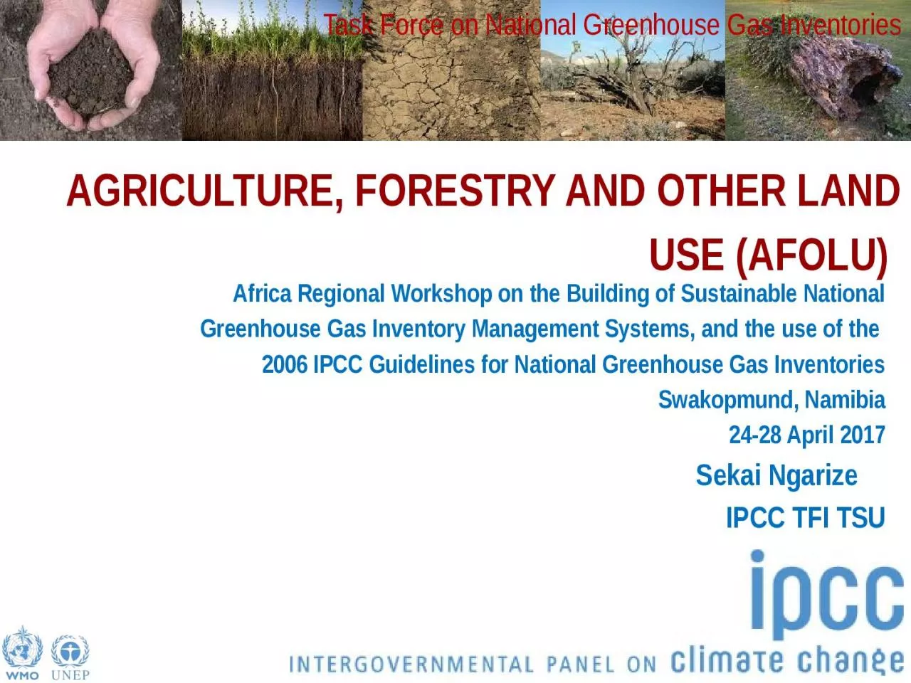
AGRICULTURE, FORESTRY AND OTHER LAND USE (AFOLU) - PowerPoint Presentation

1. AGRICULTURE, FORESTRY AND OTHER LAND USE (AFOLU) Africa Regional Workshop on the Building of Sustainable NationalGreenhouse Gas Inventory Management Systems, and the use of the 2006 IPCC Guidelines for National Greenhouse Gas InventoriesSwakopmund, Namibia24-28 April 2017Sekai Ngarize IPCC TFI TSU

2. OutlineIntroductionIPCC Guidelines for Agriculture, Forestry and Other land-use (AFOLU)AFOLU3A. Livestock3B. Land3C. Aggregate sources and non-CO2 emissions on landCross-cutting issues

3. IntroductionLivestock, Land use change and management have a significant influence on the greenhouse gas concentrations in the atmosphere. Processes covered by IPCC guidance that account for emissions and removals in the biosphere include: photosynthesis, respiration, decomposition, nitrification/denitrification, enteric fermentation, and combustion that are driven by the biological activity and physical processes.AFOLU represents 24% of net anthropogenic emissions, equivalent to about 12 Gt CO2-eq/year (AR5, 2010 GHG Inventory datasets and EDGAR).A significant proportion of GHG emissions/removals in the AFOLU sector come from developing countries.

4. Terrestrial sources/sinks of GHGsMethanogenesisPhotosynthesisMethanogenesisNitrification & denitrificationOxidationOxidation

5. Evolution of IPCC Guidance on agriculture, forestry and other land-use

6. Evolution of IPCC Guidance on Agriculture and LUCF/LULUCF

7. Agriculture, Forestry and Other Land Use (AFOLU)

8. 3a. livestock

9. 3A. Livestock emissions

10. Three methodological Tiers

11. Tier 1 - Step 1: Livestock populations (1)To calculate CH4 and N2O emissions, you first need to collect data on livestock population and MMS. To obtain this information, you should follow these steps:Assess whether a domestic livestock population exists in the country.Produce a characterization of the animal species.Calculate the annual average population (AAP).Stratify animals by annual average temperature (AAT).Collect data on manure management systems (MMS).

12. Tier 1 - Step 1: Livestock populations (2)Assess whether a domestic livestock population exists in the country. You should use:population data from official national statistics; orFAOSTAT if national data are unavailable. In FAOSTAT, data on livestock population have been directly reported by the country or estimated by FAO in case of gaps.When data available in FAOSTAT differ from official national statistics, it is good practice to contact the national focal point for FAO data to reconcile information.

13. Tier 1- Step 2: Livestock characterization

14. Tier 1 - Step 2: How to decide which livestock characterization to use?

15.

16. Step 2: Livestock population and feed characterization For higher Tier methods estimating CH4 and N2O emissions from livestock require definitions of livestock subcategories, annual populations, feed intake and characterisation. It is a good practice to identify the appropriate method for estimating emissions for each source category, and then base the livestock information (characterisation) on the most detailed requirements identified for each livestock species.Characterization may undergo iteration based on the needs assessed during the emissions estimation process.

17. Tier 1 - Step 2: Basic characterisation for livestock populations (1)Basic characterisation supporting Tier 1 requires the following information:Livestock species and categories: A complete list of all livestock populations that have default emission factor values must be developed (e.g., dairy cows, other cattle, buffalo, sheep, goats, camels, llamas, alpacas, deer, horses, rabbits, mules and asses, swine, and poultry) if these categories are relevant to the country.Annual population: Annual population data from national statistics or FAO. Adjustments should be made for seasonal births and slaughters. Annual average population should be estimated for growing population (e.g., meat animals, such as broilers, turkeys, beef cattle, and market swine)

18. Tier 1 - Step 2: Basic characterisation for livestock populations (2) Dairy cows and milk production:The dairy cow population is estimated separately from other cattle.Dairy cows are defined in this method as mature cows producing milk in commercial quantities for human consumption (FAO Production Yearbook). Sometimes dairy cows are divided into high milk producing commercial breeds and low milk producing cows. Dairy cows do not include low productivity multi-purpose cows that should be considered ‘other cattle’. Data on the average milk production of dairy cows are also required. Country-specific or FAO data may be used.Dairy buffalo may be categorized in a similar manner to dairy cows.

19. Tier 1 - Step 3: Calculate Average Annual PopulationIn the case of static animal populations (e.g. dairy cows, breeding swine, layers), estimating the AAP may be as simple as obtaining data from a one-time animal inventory. Livestock data available usually already represent the AAP, so no further calculation is needed. In the case of animal categories with a life cycle of less than one year, such as poultry, the AAP is calculated applying the following equation:Example: AAP: 60 days X 60000/365days = 9,863 chickens

20. Tier 1 - Step 4: Annual Average TemperatureStratify livestock by annual average temperature (AAT).In order to estimate CH4 emissions from manure management, the basic characterization of the animal population needs to be further stratified for the geographical location and its temperature. Estimate the percentage of the animal population located in different temperature zones. Note: Temperature has a major impact on the rate of the microbial activity that causes CH4 emissions from manure. Higher emissions rates correspond to higher temperatures rates.The temperature data should be based on national meteorological statistics where available. Countries should estimate the percentage of animal populations in different temperature zones. Where this is not possible, the AAT for the entire country can be used.

21. Tier 1 - Step 5: Manure Management Systems (1)Collect data on manure management systems (MMS).Manure (dung and urine) produced by domestic animals is usually stored in different management systems before being applied to soils as fertilizer or otherwise used for feed, fuel, or construction purposes.To estimate N2O emissions from manure management, in addition to the animal characterization, data must be collected on the fraction of manure that is managed in each type of system for each livestock category.

22. Tier 1 - Step 5: Manure Management Systems (2)IPCC provides definitions for 17 MMS in Table 10.18.IPCC provides default MCF and N2O EFs for defined MMS in Table 10.17 and Table 10.21 respectively.IPCC provides default values of cattle, buffalo and swine manure allocation per MMS (MS%) for 9 systems (Tables from 10A-4 to 10A-8):Lagoon (uncovered anaerobic lagoon).Liquid/slurry.Solid storage.Dry lot.Pit<1 month.Pit>1 month.Daily spread.Digester (anaerobic digester).Other.

23. Tier 2: Enhanced characterisation for livestock populationsThe Tier 2 livestock characterisation seeks to create relatively homogenous sub-groupings of animals dividing the population into these subcategories reflecting country-specific variations in age structure and animal performance within the overall livestock population. The Tier 2 characterisation methodology is meant to support a more accurate estimate of feed intake for use in estimating methane production from enteric fermentation by defining animals, animal productivity, diet quality and management circumstances.

24. Tier 2 - additional step: Average daily feed intake (1)The feed intake is the amount of energy an animal needs for maintenance and for activities such as growth, lactation, and pregnancy, and it is typically measured in terms of:gross energy GE (e.g., megajoules (MJ) per day) ordry matter intake DMI (e.g., kilograms (kg) per day).For all estimates of feed intake, good practice is to:Collect data on the animal’s typical diet and performance in each subcategory;Estimate feed intake from the animal performance and diet data for each subcategory.In some cases, the equations to estimate the feed intake may be applied on a seasonal basis, for example under conditions in which livestock gains weight in one season and looses weight in another (average annual population should be adjusted accordingly).

25. Tier 2 - additional step: Average daily feed intake (2)Data to be collected for estimating feed intake:Average Live-Weight (W and BW), kg; of the single animal of the sub-category [net energy for maintenance and growth (net energy for activity is used only for sheep)].Average weight gain per day (WG), kg day-1; [net energy for growth].Average Mature weight (MW), kg; The mature weight of the adult animal (when skeletal development is complete) of the inventoried group is required to define a growth pattern, including the feed and energy required for growth [net energy for growth]. At maturity as a rule W=MW.Average number of hours worked per day. [net energy for work]Feeding situation: [net energy for activity]

26. Tier 2 - additional step: Average daily feed intake (3)Data to be collected for estimating feed intake:Mean winter temperature, ºC; [net energy for maintenance of animals in colder climates]Average daily milk production, kg day-1, and fat content, %; the average daily production should be calculated by dividing the total annual production by 365 [net energy for lactation]Percent of females that give birth in a year: [net energy for pregnancy]Number of off spring produced per year: [net energy for pregnancy]Feed digestibility (DE%): The portion of gross energy (GE) in the feed not excreted in the faeces is known as digestible feed, percentage (%) of GE. Table 10.2, Volume 4, IPCC 2006. Average annual wool production per sheep, kg yr-1; [net energy for wool production]

27. Tier 2 - additional step: Average daily feed intake (4)

28. Tier 2: Gross energyTotal net energy requirement for animal performance and feed digestibility data are used to estimate the Gross Energy (GE).Gross Energy (GE) is then estimated from net energy requirement divided by feed digestibility (45-55% for low quality forage).As a QC procedure GE in energy units should be converted to dry matter intake (DMI) by dividing GE by the energy density of feed, default value 18.45 MJ kg-1 (the daily DMI should be 2-3% of the body weight of animals).

29. To be repeated for each livestock species and gasSignificant livestock species account for 25-30% or more of emissions from the source categoryDecision Tree for livestock categories

30. IPCC Methodological Guidance: Calculating emissions for Enteric Fermentation and Manure Management

31. CH4 emissions from enteric fermentation are produced during digestion of carbohydrates, which are broken down into simple molecules for absorption into the bloodstream. Ruminant livestock (e.g. cattle, sheep) are major sources of CH4, while moderate amounts are produced from non-ruminant livestock (e.g. pigs, horses). The amount of CH4 produced is a function of:type of digestive system;age of the animal;weight of the animal; andquality and quantity of food.CH4 emissions from Enteric Fermentation

32. Methodological tiers- Enteric Fermentation

33. Enteric fermentation: Calculation steps for all Tiers

34. Once you have collected data on Average Annual population (AAP) of the livestock species present in your country, you can apply equation 10.19. This is the methodology to follow.Where:Emissions = methane emissions from Enteric Fermentation, Gg CH4 yr-1EF(T) = emission factor for the defined livestock population, kg CH4 head-1 yr-1N(T) = the number of head of livestock species / category T in the countryT = species/category of livestockThen, sum emissions from all defined livestock categories to determine total national emissions from enteric fermentation. Apply equation 10.20 below:CH4 emissions from Enteric Fermentation -Tier 1 MethodWhere:Total CH4Enteric = total methane emissions from Enteric Fermentation, Gg CH4 yr-1Ei = is the emissions for the ith livestock categories and subcategories

35. CH4 emissions from Enteric Fermentation - Tier 1 Method

36. What do we do when default emissions factors are not available for all categories of livestock …For Example: Llamas are widespread in my country, but for this animal there are no default emissions factors available in the 2006 IPCC Guidelines…One approach we can follow is to develop an approximate EF using a default EF for animals with a similar digestive system. For llamas, we can approximate by using alpacas and then apply the equation below…In my country, the average live weight of llamas is 150 kg and the average alpaca weight is 65. The approximate EF for llamas is estimated from the EF of the alpaca (8 kg CH4 head-1 yr-1).1) Calculate the ratio of the weights of the animals and raise it to the 0.75 power.2) Then, multiply the ratio by a default EF for the animal with a similar digestive system. 8 = 15 kg CH4 head-1 yr-1 

37. CH4 emissions from Enteric Fermentation -Tier 1 Method - What to do when IPCC regional EFs for Dairy cows are not suitable?In case the IPCC regional default emission factor for dairy cows is considered unsuitable for the national circumstances, an alternative provided by IPCC (Vol.1, Ch.5, section 5.3.3.1 “Overlap”). To do so, you should first estimate relationship between default EF and milk yields from 2006 IPCC Guidelines, Table 10.11 and then apply it for the time series of national milk production data.For example, overlap approach to derive adjusted EFs based on national milk production (dummy data) for North America: 128 kg CH4 head-1 yr-1 divide by 8400 kg head-1 yr-1 = 0.015 (ratio).8500 kg head-1 yr-1 multiply by 0.015 = 130 kg CH4 head-1 yr-1 Average annual milk production8400850087008900EF 128130133136

38. Enteric Fermentation: Tier 2 MethodWhere:EF = emission factor, kg CH4 head-1 yr-1 GE = gross energy intake, MJ head-1 day-1Ym = methane conversion factor, per cent of gross energy in feed converted to methane. The factor 55.65 (MJ/kg CH4) is the energy content of methane Equation 10.21

39. Choice of emission factorsTier 1 method requires default EFs for the livestock categories according to the basic characterization scheme. Tier 2 methods require country-specific EFs estimated for each animal subcategory based on the gross energy intake estimated using the detailed data on animal feed and performance and methane conversion factor for the subcategory.

40. Choice of activity dataTier 1 method requires collection of livestock population data according to basic characterization.Tier 2 method requires animal population data according to single livestock enhanced characterisation depending upon the most disaggregated data requirements between enteric fermentation and manure management categories.

41. CH4 is generated during the storage and treatment of manure, produced from decomposition of manure under low oxygen or anaerobic conditions.These conditions often occur when large numbers of animals are managed in a confined area (e.g. dairy farms, beef feedlots, and swine and poultry farms), where manure is typically stored in large piles or disposed in lagoons or other types of MMS. At Tier 1 the amount of CH4 produced is a function of:number of animals;amount of manure produced; andtemperature.At higher tiers the amount is also a function of:type of MMS;portion of manure that decomposes anaerobically; andretention time.Manure Management (CH4)

42. Tier 1 method - CH4 from Manure managementFor each livestock category, calculate the emissions by multiplying the respective emission factor by the AAP, both stratified by AAT. Then, sum emissions from all defined livestock categories to determine total national emissions. (Equation 10.22, 2006GL below)Where:CH4Manure = CH4 emissions from manure management, for a defined population, Gg CH4 yr-1EF(T) = emission factor for the defined livestock population, kg CH4 head-1 yr-1N(T) = the number of head of livestock species/category T in the countryT = species/category of livestock

43. Tier 1 - CH4 from Manure management - Data for Emission factorsDefault emission factors by AAT are shown in Table 10.14, Table 10.15, and Table 10.16 in the 2006 IPCC Guidelines for the main livestock categories Default emission factors are mostly stratified by:

44. Tier 1 - CH4 from Manure management - Activity dataLivestock characterizationThis includes domestic animal species for which an IPCC default emission factor existsThis should be estimated particularly for animals like poultry with more than one life cycle per year AATThis is needed to estimate the percentage of animal population located in different temperature zonesAAPActivity data needed for the calculation of CH4 emissions from manure management are the number of animals (in terms of AAP) for each livestock category identified through the basic livestock characterisation and stratified by AAT

45. Methodological Tiers – Manure Management - CH4 emissions

46. Manure Management (CH4): calculation steps for all Tiers

47. Choice of emission factors (1)Tier 1Default methane emission factors for manure management by livestock category or subcategory are used. Default emission factors represent the range in manure volatile solids content and in manure management practices used in each region.Tier 2The Tier 2 method relies on two primary types of inputs that affect the calculation of methane emission factors from manure: manure characteristics and MMS characteristics.

48. Choice of emission factors (2) Manure characteristics includes: the amount of volatile solids (VS) produced in the manureVS can be estimated based on feed intake, digestibility (which are the variables also used to develop the Tier 2 enteric fermentation emission factors) and ASH content in the manure. the maximum methane-producing capacity of the manure (Bo)Bo varies by animal species and feed regimen and is a maximum theoretical methane yield based on the amount of total as-excreted VS in the manure. Manure management system characteristics includes: the types of systems used to manage manure and a system-specific methane conversion factor (MCF) that reflects the portion of Bo that is achieved. Regional assessments of MMS are used to estimate the portion of the manure handled with each.

49. Choice of emission factors (3)For Tier 2 method while some default values have been provided in the IPCC Guidelines, country-specific values of parameters Bo, VS, MCF and manure allocation per MMS should be used as far as possible as the default values may not encompass the potentially wide variations in these values according to national circumstances.

50. Choice of activity dataTier 1 method requires collection of livestock population data according to basic characterization.Tier 2 method requires two main types of activity data: animal population datasingle livestock enhanced characterisation depending upon the most disaggregated data requirements between enteric fermentation and manure management should be adopted. regional population breakdown according to for each major climatic zone along with the average annual temperature to select the EFsMMS usage dataportion of manure managed in each MMS for each representative animal species from published literature, national surveys, expert judgement etc.

51. Tier 2 - CH4 from Manure managementWhere:EF(T) = annual CH4 emission factor for livestock category T, kg CH4 animal-1 yr-1VS(T) = daily volatile solid excreted for livestock category T, kg dry matter animal-1 day-1365 = basis for calculating annual VS production, days yr-1Bo(T) = maximum methane producing capacity for manure produced by livestock category T, m3 CH4 kg-1 of VS excreted0.67 = conversion factor of m3 CH4 to kilograms CH4MCF(S,k) = methane conversion factors for each manure management system S by climate region k, %MS(T,S,k) = fraction of livestock category T's manure handled using manure management system S in climate region k, dimensionlessEquation 10.23

52. Manure Management (N2O) N2O is produced, directly and indirectly, during the storage and treatment of manure before it is applied to land or otherwise used for feed, fuel, or construction purposes.Direct N2O emissions occur via combined nitrification and denitrification of nitrogen contained in the manure.Indirect emissions result from volatile nitrogen losses that occur primarily in the forms of ammonia and NOx. The fraction of excreted organic nitrogen that is mineralized to ammonia nitrogen during manure collection and storage depends primarily on time, and to a lesser degree temperature.

53. Manure Management: Direct (N2O) N2O is emitted directly into the atmosphere during the storage and treatment of manure via combined nitrification and denitrification of N contained in manure. N2O emissions are a function of: N content of manure;duration of storage; andtype of treatment.

54. Calculation steps for all Tiers

55. Manure Management: Direct (N2O) Tier 1Once you have collected data on the fraction of manure managed within different management systemsNOTE: This information is useful to calculate direct and indirect emissions of N2O. This is the methodology to follow.For each MMS, you need to multiply the total amount of N excretion (from all livestock species/categories) managed in it by an emission factor for that type of MMS. Apply: Equation 10.25 (2006 GL) (see next slide)Then, sum emissions over all MMS to obtain the total national emissions.

56. Manure Management: Direct (N2O) Tier 1 (1)Direct N2O emissions from manure management is given by Where:N2OD(mm) = Direct N2O emissions from Manure Management in the country, kg N2O yr-1N(T) = number of animals/category T in the countryNex(T) = annual average N excretion/head of species/category T, kg N animal-1 yr-1MS(T,S) = fraction of total annual N excretion for each livestock species/category T handled in MMS, S in the country, dimensionlessEF3(S) = EF for direct N2O emissions from MMS, S in the country, kgN2O-N/kg N in MMS, SS = manure management systemT = species/category of livestock44/28 = conversion of (N2O-N)(mm) emissions to N2O(mm) emissionsEQUATION 10.25 (2006 GL)

57. Manure Management: Direct (N2O) Tier 1 (2) Lets review the equation in more detail: =N(T)Nex(T)EF3 (S)MS(T,S)NEmms = total N excretion for each MMS per year N2OD(mm) ] STN(T)This is the AAP expressed in number of head of animal category T. This data can be obtained from official national statistics or, if not available, from the FAOSTAT Emissions database.Nex(T)This is the annual average N excretion expressed in kg N per head of animal category T.MS(T,S)This is the fraction of total annual N excretion for each animal category T managed in a MMS S, dimensionless.

58. You can estimate the annual N excretion using the equation 10.30Nex(T) = Nrate(T) • • 365 Manure Management: Direct (N2O) Tier 1 (3)

59. Manure Management: Direct (N2O) Tier 1 (4) - The MMS usage data can be obtained:MS(T,S)From national statistics, independent surveys or expert judgementThe best means of obtaining MMS system usage data is to consult regularly published national statistics. If such statistics are unavailable, the preferred alternative is to conduct an independent survey of MMS system usage. If the resources are not available to conduct a survey, experts should be consulted to obtain an opinion of the system distribution.From default valuesIf country-specific MMS usage data are not available, default values should be used. ​The IPCC default values for dairy cows, other cattle, buffalo, swine (market and breeding swine), and poultry should be taken from Tables 10A-4 through 10A-8 of Annex 10A.2 of the 2006 IPCC Guidelines.

60. Manure Management: Direct (N2O) Tier 1 (5)EF3(S) – Once the value of total N excretion is known, then the total amount of N excretion (from all livestock categories) in each manure management system needs to be multiplied by an emission factor, defined for each manure management system.Default emission factors for each MMS are available in Table 10.21 of the 2006 IPCC Guidelines and are expressed as kg N2O-N/kg N excreted. For example, the emission factor for manure management "Solid storage" is 0.005.

61. Manure Management: Direct (N2O) Tier 1Finally, the equation needs to be multiplied by this conversion factor…44/28…WHY?EF3(S) are expressed in terms of amount of nitrogen (N2O -N). ​In order to obtain the amount of N2O emissions the value should be multiplied by 44/28 where:​44…is the molecular weight of N2O [(14 • 2) + 16]28…is the molecular weight of N2 (14 • 2)To be multiplied by 10-6 to convert in Gg

62. Choice of emission factors Tier 1 Annual nitrogen excretion for each livestock category defined by the livestock population characterisation.Country-specific values or from other countries with livestock with similar characteristicsIPCC defaults of N excretion rates (2006 IPCC Guidelines) could be used with typical animal mass (TAM) valuesDefault emission factors from the IPCC Guidelines

63. Choice of emission factors Tier 2Annual nitrogen excretion for each livestock category defined by the livestock population characterisation based on total annual N intake and total annual N retention data of animals.Country-specific emission factors that reflect the actual duration of storage and type of treatment of animal manure in each system

64. Choice of activity dataTier 1 Animal population data according to basic characterization.Default or country specific manure management system usage dataTier 2Animal population data according to single enhanced characterization. Country-specific manure management system usage data from national statistics, independent survey or expert judgement

65. 3b. land

66. Outline - FOLUDefinition of basic conceptsSteps in preparing inventory estimatesCarbon pools definitionsLand use categoriesApproaches to land representation and activity data (AD)Land Representation: Why we need Land StratificationGeneric Methodological Guidance for All Land CategoriesMethodological approaches used in the estimation of emissions/removals in FOLU sectorCross-cutting issuesExercise

67. Steps in a LULUCF Inventory Preparation

68. Definition of ConceptsThe land sectors is made of:Emissions to the atmosphere GHG caused by losses of organic matter from terrestrial ecosystems…and of carbon dioxide (CO2) removals from the atmosphere as uptake by vegetation and stored in the organic matterOrganic matter is composed of organic compounds that are part of organisms such as plants and their remains. It is essentially composed of the four elements below; their weight in organic matter is also provided.Carbon (C) 40-55%Oxygen (O) 35-45%Hydrogen (H) 3-5%Nitrogen (N)1-4% %These elements are constituents of the three important GHGs, that are reported in the land use sector, namely:Carbon Dioxide (CO2),Methane (CH4)Nitrous Oxide (N2O)

69. Stratification of organic matter within 6 carbon poolsCarbon PoolsSince C is the most relevant component of the organic matter. The amount of organic matter in an ecosystem is regarded as a carbon stock (C Stock) that can be stratified into six so-called carbon pools present in the below image. Carbon Pool: is a reservoir, that is component of the climate system where a GHG or a precursor of a GHG is stored. In particular carbon pools have the capacity to accumulate and release carbon dioxide.5Soil Organic Matter (SOM)6Harvested Wood Products (HWP)Living Biomass (LB) includes:1Above-Ground Biomass (AB)2Below-Ground Biomass (BB)Dead Organic Matter (DOM) includes:3Dead Wood (DW)4Litter (LI)

70. IPCC Guidance on DOM and Soil C

71. C stocks in C poolsC stock is the amount of C contained in the organic matter and is calculated by multiplying the organic matter by a conversion factor also referred as Carbon Fraction (CF); it is usually expressed in tonnes. To convert dry organic matter into carbon, the IPCC Guidelines provides default carbon fraction values for the below C pools.Living Biomass:Table 4.3, Volume 4, 2006 IPCC Guidelines for Forest Land0.5 for woody biomass and 0.47 for herbaceous biomass for Grassland (page 6.29. Volume 4, 2006 IPCC Guidelines)0.5 for Flooded Lands (Equation 7.10, Volume 4, 2006 IPCC Guidelines)0.5 for Settlements (page 8.9, Volume 4, 2006 IPCC Guidelines)Litter:0.37 (from Equation 2.19, Volume 4, 2006 IPCC Guidelines)0.4 for Cropland, Grassland and Settlements (pages 5.14,6.11, 8.21, Volume 4, 2006 IPCC Guidelines)Dead wood:0.50 for Cropland, Grassland and Settlements (pages 5.14, 6.11, 8.21, Volume 4, 2006 IPCC Guidelines)SOM in mineral soils: 0.58 (page 2.38, Volume 4, 2006 IPCC Guidelines)Peat: Table 7.5, Volume 4, 2006 IPCC Guidelines

72. C stocks in C poolsC pools exchanges GHG as removals from the atmosphere through photosynthesis and as emissions to the atmosphere through biochemical processes (decay of C stocks) and physiochemical process (fires).Emissions occur as C stock losses from C pools while removals occur as C stock gains. Consequently C stock changes are a proxy for estimating GHG emissions/removals for land categories.Both, C stock gains (positive sign) and C stock losses (negative sign) are multiplied by -44/12 to convert them in CO2 removals and emissions respectively. Where 44 is the molecular weight of CO2 and 12 is the atomic weight of C.Further, transfers (as gains or losses) of organic matter among C pools occur as a consequence of mortality (natural and man-made) and decay, so determining C stock losses in the C pools from which the stock is transferred and C stock gains in the pools in which the C stock is transferredBiomass is the only sink among C pools

73. Carbon cycle processes: showing carbon stock flows into and out of carbon pools Living BiomassCountries can choose to account for HWP poolDead Organic Matter

74. The use of managed land as a proxy in estimating land-based emissions and removals (E/R)Factors governing E/R can be both natural and anthropogenic and can be difficult to distinguish between causal factorsInventory methods have to be operational, practical and globally applicable while being scientifically soundIPCC Guidelines have taken the approach of defining anthropogenic greenhouse gas emissions by sources and removals by sinks as all those occurring on ‘managed land’‘Managed land is land where human interventions and practices have been applied to perform production, ecological or social functions’Managed land has to be nationally defined and classified transparently and consistently over timeGHG emissions/removals need not be reported for unmanaged land

75. Six land-use categoriesOther landForest LandSettlementsWetlandCroplandGrasslandStock changes of C pools are estimated and reported for the six “top-level” land-use categories Subdivide according to national circumstances

76. Land-use subcategories and carbon poolsEach land-use category is further subdivided into land remaining in that category (e.g., FL-FL) and land converted from one category to another (e.g., FL-CL) for estimation of C stock changes. The total CO2 emissions/removals from C stock changes for each LU category is the sum of those from these two subcategories.

77. Total estimates for GHG are made up of subdivisions of land use categoriesTotal emissions from land use categoryLand remaining in the same land use categoryLand converted from one category to that category

78. Land RepresentationIn the 2006 GL Land representation is the analysis undertaken to identify and quantify human activities on land, as well as to track their changes over time. This includes analysis of information, on land classification, land area data, and sampling that represents various land-use categories, this information is needed to estimate the carbon stocks, and the emission and removal of greenhouse gases associated with Forestry and Other Land Use (FOLU) activities.The land representation results in a stratification of the total area of the country into strata (units of land) homogeneous for a number of variables, that explain the current level and dynamic of C stocks within the stratum, with the purpose of making the GHG inventory compilation practicable while enhancing accuracy of GHG estimates.Land is characterized by bio-physical variables and various human activities. The variables for land stratification are listed below:Biophysical characteristicsLand UseManagement practices and disturbancesOther category specific variablesStratum: Unit of Land

79. Land Representation: Why we need Land StratificationWhen estimating GHG emissions and removals, land areas are used as activity data (AD). As activity data, they represent the magnitude of a human activity that generates GHG emissions and/or removals during a given period of time.This is why the stratification of land is a paramount tool to achieve accuracy of GHG estimates. Example of a land representation and associated C stock changes below. This illustration below is an example of how land stratification correlates with the amount of C stocks found in a unit of land and their dynamic. Forest Land CroplandAs you can see the conversion of land from forest land to cropland determines a negative C dynamic of C stocks (i.e. the amount of C stocks in this unit of land decreases across time).

80. Land Stratification – Bio-physical characteristics (1) IPCC provide guidance for land stratification according to a number of variables as provided in previous slides (slide 83). IPCC Land stratification by the biophysical characteristics variables include: ClimateEcological Zone Soil TypeBio-physical characteristics impact annual C stock gains and losses as well as the C stocks carrying capacity of landThe stratification of land by climate is important because temperature and water are the two main parameters that determine the accumulation of biomass and decay of organic matter on the land. The IPCC recommends classifying land according to climate zones that are defined by a set of rules based on: Annual mean daily temperatureTotal annual precipitationTotal annual potential evapo-transportation (PET)ElevationThe list of climate zones covering most managed lands:BorealCold temperate dry Cold temperate wetWarm temperate dryWarm temperate moistTropical dry Tropical moist Tropical wet

81. Land Stratification – Bio-physical characteristics (2) The stratification of land by ecological zone (or potential vegetation zone) is important since woody biomass is the second largest terrestrial C pool. The IPCC uses the Global Ecological Zone (GEZ) classification provided by the Food and Agriculture Organization (FAO) of the United Nations. Below are ecological zones provided by FAO:Tropical rainforestTropical most deciduous forestTropical dry forestTropical shrublandTropical desertTropical mountain systemsSubtropical humid forestSubtropical dry forestSubtropical steppeSubtropical desertSubtropical mountain systemsTemperate oceanic forestTemperate continental forestTemperate steppe Temperate desert Temperate mountain systemsBoreal coniferous forestBoreal tundra woodlandBoreal mountain systemsPolar

82. Land Stratification – Bio-physical characteristics (3) The stratification of land by soil type is important because soil contains the largest portion of terrestrial C stocks in the Soil Organic Matter (SOM) carbon pool. Soil Organic Carbon (SOC) level and dynamic are influenced by the physical and bio-chemical characteristics of soil. The 2006 IPCC Guidelines classify country’s soils in default types derived from the World Harmonized Soil Database. IPCC provides methodological guidance on two soil types namely organic and mineral soils.

83. Land Stratification – Land UseIPCC provides guidance on stratifying land use in the following order: Managed and unmanaged landSix IPCC land use categories“Land remaining in the same land-use category” and “Land converted into a new land use category” Land conversion categoriesManaged land are stratified (land use categories) according to their current land use (i.e. Forest land, Cropland, Grassland, Wetlands, Settlements, Other land), and changes in use over time. (second step)Unmanaged lands are stratified (land use categories) according to their current cover (i.e. Forest land, Grassland, Wetlands, Other land)

84. Land Stratification – Land UseCan countries apply their own country specific land use definitions?Yes- countries may apply their own country specific definitions as long as:a hierarchical order is established among the country specific definitionsCountry specific definitions need to cover the entire range of land uses represented in the country’s territory and avoid mixing areas with very different C stocks and C stock dynamics together in the same category For example, the combination of both types of land, without C stocks (such as sands) and with significant C stocks (such as steppe), must be avoided.Often country-specific definitions are based on land cover classes, and therefore need to be reconciled with IPCC land use categories.For example FAO publishes area data on forest (FRA database) and non-forest categories (FAOSTAT database) such as arable land, permanent crops, etc.

85. Land Stratification – Land Use Change (1)The third step is to differentiate the land use categories according to their historical land uses. Changes from a land use category to another causes changes in the level of C stocks (abrupt impact) and determines a dynamic in C stock changes across a transition period (lagged impact). This means that land use history is an important factor when selecting the appropriate methodology for estimating GHG emissions and removals. Consequently, the IPCC stratifies land use category areas in two types shown here.Land remaining in a land use category (no conversion in the last 20 years)Land converted into a new land use category (conversion within the last 20 years)

86. Land Stratification – Land Use Change (2)Land conversion process:The conversion process is tracked across a 20-year “transition period” (IPCC default). In such a period, the C stocks dynamic in the land conversion category (e.g. GL-FL) is different than the dynamic in the corresponding land remaining category (e.g. FL-FL). Information on historical land use allows the application of different stock change factors according to different types of conversion. If the land use has not changed in the last 20 years, the land is reported under the category “Land remaining under the same land use.” If the land use has changed in the last 20 years, the land is reported under the category “Land converted to the new land use” and in the relevant subcategory. The fourth step is to differentiate land conversion categories according to the previous land use in the 30 land use change sub-categories. E.g. Forest land converted to Cropland

87. Land stratification – Land use versus Land coverUsing the example of an area covered by trees that is clear cut will help to understand the methodological difference between land cover and land use.Applying a land cover classification, we may just estimate the loss of the biomass C stock of the tree cover. While applying a land use classification, we will estimate:The loss of the biomass C stockThe gain of biomass C stock associated with the following vegetation regrowth (the type of which depends from the current land use e.g. forest regrowth in case of temporary loss of forest cover).The change in the DOM C stock as difference between the C stocks in the previous and in the current land use.The change in SOC as difference between the C stocks in the previous and in the current land use.

88. Land stratification – Management system/practices and disturbancesThis table illustrates a list of default management systems/ practices provided by the IPCC guidelines. The table reports which C pools are most affected by various management systems/practices and by their changes.The stratification by the management system/ practices on land is a good proxy for the expected level and dynamic of C stocks, and therefore it can also be used as a further level of land stratification. Stratification by management system is required especially for the soil organic matter (SOM).

89. Land stratification – DisturbancesThe frequency of fires in an ecosystem is a variable for stratification since it impacts the average long term C stocks, as well as the annual dynamic of C stocksOther common disturbances are insects, pests and wind. The variable for stratification by disturbances that applies to all land categories is fire. Fires can occur as a consequence of human activities and/or of natural events. Prescribed fires and wildfires should both be taken into account in the GHG Inventory when occurring on managed land.

90. Consistent land representation – Methodological ApproachesConsistency in land representation is key to ensure that no artefact trends in GHG estimates are caused by incomplete/inconsistent time seriesThe level of aggregation at which the land representation should be reported in the NGHGI is that of land use categories (the six land remaining categories and the associated thirty land-use change categories). Approaches for land representation are applied to classify the territory, according with the stratification scheme applied, and to quantify the area of each unit of land.A combination of approaches can be used to better adapt to data availability over time and space. Although, to ensure consistency of land representation, each unit of land identified must be reported with the same approach across the entire time series.The most efficient tactic to build a consistent land representation is to apportion the land in macro-units of land homogeneous for climate, ecological zone and soil and to build a land representation for each of the macro-units.

91. Three approaches for Consistent Land Representation: Methodological Approaches

92. 92Approach 1

93. Approach 2 93

94. Approach 3: Spatially Explicit94

95. Ex. # 1: Land Use matrix: Can you fill in the missing values? Initial Final FL CLGLWLSEOLFinal AreaFL502 6 020??CL5 35 8 0 2 0 50GL3 7 ?? 0 0 0 37WL 800203031SE0 00032032OL0 000055Initial Area66 44??20??5215

96. And the answer is… Initial Final FL CLGLWLSEOLFinal AreaFL502 6 02060CL5 35 8 0 2 0 50GL3 7 27 0 0 0 37WL 800203031SE0 00032032OL0 000055Initial Area66 444120395215

97. Consistent land representation – Reporting (1)Reporting - Annual matrices of land use and land use changeLet’s identify how matrices are complied, what information they contain and what they look like by following the example below.Inventory year is Country X has been subdivided in a number of strata homogeneous by climate zone, ecological zone and soil type.Then, for each stratum a time series of annual matrices has been prepared as shown in the below matrices. For instance, a stratum could be: Warm Temperate Moist climate zone (WTM), Temperate Mountain Systems ecological zone (TMS), and High Activity Clay soil type (HAC). As reported in the example below:

98. Consistent land representation – Reporting (2)Inventory year is How should I read matrices?Note that a time series is composed by a number of tables corresponding to the number of years for which the land representation has to be built plus 19. For example, the time series for the GHG inventory period 2005-2017 will be composed by 30 annual matrices (i.e. from matrix 1985-1986 till matrix 2015-2016)Finally, data reported in the time series of annual matrices (1 time series for each combination of climate zone, ecological zone and soil type) are then aggregated according to GHGI category reporting (i.e., in land use and land-use change categories).2006

99. Generic Methodological Guidance for All Land Categories

100. The IPCC Guidelines make two assumptions: A) Cflux = ∆Cstocks B) Change in carbon stocks can be estimated from land use/change and management at various points in time, their impacts on carbon stocks and the biological response to them. (IPCC 2006 GL, page1.6, section 1.2.1, para 3)A simple first order approach in the IPCC Guidelines

101. Generic Methodological Approaches to Estimating C Stocks Changes on Managed Land

102. Generic Approaches to Estimating C Stocks Changes on Managed Land: CO2 Emissions from C stock changes on landAnnual carbon stock changes as sum for all land use categories: Equation 2.1 (2006 GL, pg 2.6)Annual C stock changes for a land-use category - sum of each stratum within category: Equation 2.2 (2006 GL, pg 2.7) Annual carbon stock changes for a stratum of a land-use category - sum of all carbon pools: Equation 2.3 (2006 GL, pg 2.7)ΔCLUi = ΔCAB + ΔCBB + ΔCDW + ΔCLI + ΔCSO ΔCLAND = ΔCFL + ΔCCL + ΔCGL + ΔCWL + ΔCSL+ ΔCOL ΔCLU = Σ ΔCLU i

103. Generic approaches when estimating C stock changes (1)In the land use sector, carbon stock changes are estimated to derive emissions and removals of CO2, CH4 and N2O in each GHG inventory category. The C stock changes in each category of the land use sector are estimated for each carbon pool by using two generic methodological approaches different and equally valid to estimating C stock changes as shown below. Method 1 Method 2Gain and Loss Method is a the process-based approach, which estimates the net balance of C stock additions to and removals from a carbon pool.Stock Difference Method is a stock-based approach, which estimates the difference in C stocks at two points in time.

104. Generic approaches when estimating C stock changes (2)Carbon Stock in year 1Carbon Stock in Year 2Difference between carbon stocks (Stock-Difference Method)Land Use typeSum of gains and losses (Gain-Loss Method)C uptake through GrowthHarvestDisturbances12

105. Stock-Difference MethodStock-Difference Method can be used where carbon stocks in relevant pools are measured at two points in time to assess carbon stock changesC stock changes are estimated from measurements of C stocks at periodic intervals (t1, t2, …, tn) in the same area (i.e. area across which measuring C stocks at times t1 and t2 must be the same and be equivalent to the area of the stratum at the latest date i.e. t2). The Stock-difference is often used with time series of national forest inventory data.Where:ΔC = annual carbon stock change in the pool, tonnes C yr-1C1 = carbon stock in the pool at time t1, tonnes CC2 = carbon stock in the pool at time t2, tonnes CEquation 2.5 page 2.10, Vol 4, 2006GL should be used for each land stratum when using the Stock-Difference Method.∆C = (C2 – C1 )/(t2 – t1)

106. Gain-Loss Method Gains-Loss Method involves tracking inputs and outputs from a C pools: e.g., gains from growth (increase of biomass) and transfer of carbon from another pool (e.g., transfer of carbon from the live biomass carbon pool to the dead organic matter pool due to harvest or natural disturbances) and loss due to harvest and mortality. ΔC = annual carbon stock change in the pool, tonnes C yr-1 ΔCG = annual gain of carbon, tonnes C yr-1 ΔCL = annual loss of carbon, tonnes C yr-1Equation 2.4, page 2.9, Vol 4, 2006 GL∆C = ∆CG – ∆ CL

107. Biomass: Land Remaining in a Land-use Category Carbon stock change in biomass on Forest Land is likely to be an important sub-category due to substantial fluxes arising from management and harvest, natural disturbances, natural mortality and forest regrowth.Changes in C stocks in biomass pool can be estimated using either Stock-Change or Gain-Loss method. The Gain-Loss Method requires the biomass carbon loss to be subtracted from the biomass carbon gain.Gain-Loss Method is the basis of Tier 1 method, for which default values for calculation of increment and losses are provided in the IPCC Guidelines.

108. Gain & Loss method for Biomass C pool - Tier 1The default IPCC method (Tier 1) for estimating biomass C stock changes (above-ground and below-ground) in a land remaining in a land-use category is to use Gain and loss method which is formulated using the equation 2.7: The two elements in equation 2.7 are the annual increases (ΔCG) and decreases in biomass due to biomass growth and loss (ΔCL) . ΔCG = Σ i, j (Ai,j GTOTALi,j CFi,j) (Equation 2.9)ΔCL = Lwood−removals + Lfuelwood + Ldisturbance (Equation 2.11)

109. Annual increase in biomass carbon stocks (Gain-Loss Method), ΔCG – (Land remaining in same land use category) ΔCG = Σ i, j (Ai,j GTOTALi,j CFi,j)Where:ΔCG = annual increase in biomass carbon stocks due to biomass growth in land remaining in the sameland-use category by vegetation type and climatic zone, tonnes C yr-1A = area of land remaining in the same land-use category, haGTOTAL= mean annual biomass growth, tonnes d. m. ha-1 yr-1i = ecological zone (i = 1 to n)j = climate domain (j = 1 to m)CF = carbon fraction of dry matter, tonne C (tonne d.m.)-1Equation 2.9, page 2.15, Vol 4, 2006 GL

110. Average annual increment in biomass (GTOTAL): Tier 1Where:GTOTAL = average annual biomass growth above and below-ground, tonnes d. m. ha-1 yr-1GW = average annual above-ground biomass growth for a specific woody vegetation type, tonnes d. m. ha-1 yr-1R = ratio of below-ground biomass to above-ground biomass for a specific vegetation type, in tonne d.m. below-ground biomass (tonne d.m. above-ground biomass)-1(Equation 2.10, page 2.15, Vol 4, 2006 GL). GTOTAL = Σ{GW • (1+ R)}

111. Gain & Loss method for Biomass C pool – Tier 1Using the gain-loss method at Tier 1, the annual increase in Living Biomass (∆𝐶𝐺 perennial biomass) is the sum of each land stratum (i,j) gain. The annual increase in Living Biomass is calculated by using estimates of the area and either the default mean annual biomass growth rates, or, the average annual above-ground biomass growth rates together with the root-to-shoot ratio (R). These elements form equations 2.9 and 2.10 (2006GL) shown below.

112. Average annual increment in biomass (GTOTAL): Tier 2 & 3 GTOTAL = Σ{IV • BCEFI • (1+ R)}IV = average net annual increment for specific vegetation type, m3 ha-1 yr-1BCEFI = biomass conversion and expansion factor for conversion of net annual increment in volume(including bark) to above-ground biomass growth for specific vegetation type, tonnes above-groundbiomass growth (m3 net annual increment)-1 (Equation 2.10, page 2.15, Vol 4, 2006 GL).

113. Biomass carbon stocks losses (Gain-Loss Method), ΔCL ΔCL = Lwood−removals + Lfuelwood + LdisturbanceThe annual decrease in C stocks due to biomass losses (∆𝑪𝑳) in a land remaining in the same land-use category are estimated applying equation 2.11. The losses in biomass are due to, harvesting of wood (roundwood removals), fuelwood and disturbances,Where:ΔCL = annual decrease in carbon stocks due to biomass loss in land remaining in the same land-use category, tonnes C yr-1Lwood-removals = annual carbon loss due to wood removals, tonnes C yr-1 Lfuelwood = annual biomass carbon loss due to fuelwood removals, tonnes C yr-1Ldisturbance = annual biomass carbon losses due to disturbances, tonnes C yr-1(Equation 2.11, Vol 4, Page 2.16 , 2006 GL)

114. Gain & Loss method for Biomass C pool – Wood RemovalsBiomass C stock losses associated with industrial roundwood removals are estimated by applying the following equation (2.12 , 2006GL):If country-specific data on industrial roundwood removals (H) are not available, FAO data should be used. However, the FAO data exclude bark, while BCEF (as well as BEF) are built for industrial roundwood including bark. To expand FAO data to industrial roundwood including bark, the expansion factor 1.15 is applied. Once expanded to over bark industrial roundwood, the FAO data can be used in equation 2.12

115. Gain & Loss method for Biomass C pool – Fuel wood Biomass C stock losses associated with fuelwood gathering are estimated applying the following equation 2.13 (2006 GL):National statistics on wood harvest can report both industrial roundwood and fuelwood removals together. In such a case, wood harvest has to be apportioned to equations 2.12 and 2.13, according to an available proxy (i.e. wood bioenergy statistics) or expert judgement.

116. Gain & Loss method for Biomass C pool – DisturbancesBiomass C stock losses due to disturbances are estimated by applying the following equation 2.14 (2006GL):At higher Tiers, it is good practice to compile all C stock changes (C stock transfers and carbon emissions) in a disturbance matrix to ensure mass conservativeness in reporting (see page 2.19 Table 2,1 (2006 GL) for an example of a disturbance matrix)

117. Ex. # 2: Can you find the biomass C pool loss/gain?Growth = 200,000 tonnes C yr-1Fuelwood removals = 300 tonnes C yr-1 Natural disturbance losses= 2000 tonnes C yr-1 Loss due to Harvest = 500 tonnes C yr-1

118. And the answer is…ΔCG = 200,000 tonnes C yr-1ΔCL = Lwood −removals + Lfuelwood + Ldisturbance = 500 + 300 + 2000 = 2800 tonnes C yr-1 ΔCbiomass = ΔCG – ΔCL = 200,000 – 2800 = 197200 tonnes C yr-1

119. Stock Change Method∆C = (C2 – C1)/(t2 – t1)C = total carbon in biomass for time t1 to t2 [i = ecological zone i (i = 1 to n)j = climate domain j (j = 1 to m)]A = area of land remaining in the same land-use category, ha (see note below) V = merchantable growing stock volume, m3 ha-1R = ratio of below-ground biomass to above-ground biomass, tonne d.m. below-ground biomass (tonne d.m. above-ground biomass)-1CF = carbon fraction of dry matter, tonne C (tonne d.m.)-1BCEFS = biomass conversion and expansion factorEquation 2.8 a and b, page 2.12, Vol 4, 2006 GL - ( land remaining in same land use category) C = Σi,j(Ai,j●Vi,j●BCEFSi,j●(1+Ri,j)●CFi,j)

120. Biomass: Land Converted to Other Land-Use Category – ( Tier 2 and 3) ΔCB = ΔCG + ΔCCONVERSION − ΔCLWhere:ΔCB = annual change in carbon stocks in biomass on land converted to other land-use category, in tonnes C yr-1ΔCG = annual increase in carbon stocks in biomass due to growth on land converted to another land-usecategory, in tonnes C yr-1ΔCCONVERSION = initial change in carbon stocks in biomass on land converted to other land-use category, in tonnes C yr-1ΔCL = annual decrease in biomass carbon stocks due to losses from harvesting, fuel wood gathering and disturbances on land converted to other land-use category, in tonnes C yr-1 (Equation 2.15, page 2.20, Vol 4, 2006 GL)

121. Gain & Loss method for Biomass C pool in land under conversionBiomass carbon stock changes in a land converted to a new land-use category, the IPCC default methodology uses a similar equation (Land remaining in same category) except with the addition of a third factor to calculate the abrupt C stock change associated with conversion (ΔCCONVERSION ). Please note that at Tier 1, in case of perennial vegetation the C stock of biomass (CB) in a land converted to a new land-use category is equal to the sum of annual ∆𝐶 calculated with equation 2.15.Net C stock change associated with conversion is estimated in the year of conversion only, by using equation 2.16 (2006 GL) ( see next slide)

122. Initial change in biomass carbon stocks in Land Converted to Other Land-Use Category * ΔCCONVERSION = Σi(BAFTER – BBEFORE) ● ΔATO OTHERS i ● CFWhere:ΔCCONVERSION = initial change in biomass carbon stocks on land converted to another land category, tonnes C yr-1BAFTERi = biomass stocks on land type i immediately after conversion, t d.m.ha-1BBEFOREi = biomass stocks on land type i before conversion, t d.m. ha-1ΔATO_OTHERSi = area of land use i converted to another land-use category in a certain year, ha yr-1CF = carbon fraction of dry matter, tonne C (t d.m.)-1i = type of land use converted to another land-use category (Equation 2.16, Page 2.20, Vol 4, 2006 GL)

123. Change in C stocks in DOM: Land Remaining in the same land use categoryThe Tier 1 assumption for both dead wood and litter pools for all land-use categories is that their stocks are not changing over time if the land remains within the same land-use category.Tier 2 methods for estimation of carbon stock changes in DOM pools calculate the changes in dead wood and litter carbon pools by either Gain-Loss Method or Stock-Difference Method (GPG LULUCF provides guidance on DOM only for FL)These estimates require either detailed inventories that include repeated measurements of dead wood and litter pools, or models that simulate dead wood and litter dynamics.

124. Gain-Loss MethodA = area of managed land,ha DOMin = average annual transfer into DW/litter pool (due tomortality, slash due to harvest and natural disturbance),t d.m./ha/yrDOMout = average annual transfer out of DW/litter pool, t d.m./ha/yrCF = carbon fraction of dry matter, tC/(t d.m.)(Equation 2.18, page 2.23, Vol 4, 2006 GL)∆CDOM = [A ●(DOMin – DOMout)] ● CF

125. Stock-Difference MethodA = area of managed land, ha DOMt1 = DW/litter stocks at time t1 for managed land, t d.m/haDOMt2 = DW/litter stocks at time t2 for managed land, t d.m/haT = (t2-t1) = time period between the two estimates of DOM, yrs.CF = carbon fraction of dry matter, t C/(t d.m.) (Equation 2.19, Page 2.23, Vol 4, 2006 GL)∆CDOM = [A ●(DOMt2 – DOMt1 )/T] ● CF

126. Change in C stocks in DOM: Land Converted to Other Land-use The Tier 1 assumption is that DOM pools in non-forest land categories after the conversion are zero, i.e., they contain no carbon. The Tier 1 assumption for land converted from forest to another land-use category is that all DOM carbon losses occur in the year of land-use conversion. For land converted to Forest Land litter and dead wood carbon pools starting from zero carbon in those pools. DOM carbon gains on land converted to forest occur linearly, starting from zero, over a transition period (default assumption is 20 years)

127. In summary, at Tier 1, Biomass C stock changes must be estimated for:Forest land remaining forest landCropland remaining Cropland, limited to perennial cropsEach land use conversion from and to Forest land, Cropland, GrasslandIn any other land use and land-use conversion Biomass C stocks are assumed to be not significantIn summary, at Tier 1, DOM C stock changes must be estimated for:Each land use conversion from and to Forest landIn Forest land remaining Forest land DOM C stocks are assumed to be at long term equilibrium.In any other land use and land-use conversion DOM C stocks are assumed to be not significantBiomass and DOM C stock changes

128. Land remaining Land categories:Tier 2 method:No C pool is assumed constant (except for OL)Country-specific parameters with more disaggregated ADStock-Difference method Land converted categories:Tier 2 method:No C pools is assumed constant.C stocks before and following conversion can be non-zero. Country-specific parameters and more disaggregated AD.Tier 3 method: nationally specific complex methods involving modelling and/or measurementsBiomass and DOM C stock changes

129. Estimates of carbon emissions and removals involve the multiplication of activity data and emission factors:The amount of area undergoing a specific transition- this is called the Activity DataThe change in carbon pools association with that transition- this is called the Emissions FactorExamples of IPCC biomass default valuesThe default carbon fraction = 0.47 Source: IPCC (2006) – Examples of default values for AGB and ABG increment taken from Tables 4.7, 4.8, 4.9, and 4.10

130. IPCC Tier 2 Biomass Values of Country XX Note: To convert Biomass to carbon stock (tC/ha), multiply for example for Evergreen Forest type ABG: 238.23 by 0.48 (CF) = 114.35 tC/ha and then convert tonnes of carbon per ha to CO2 emissions; multiply 114.35 by 44/12 = 419.28 tCO2/ha( IPCC default carbon fraction is 0.47, this can be variable as you can see in above example country specific values are 0.47-0.48)

131. Soil Organic Matter - SOMSoil Organic Carbon (SOC) accumulates in the soil mainly from decomposition processes of plant tissues whose organic matter (dead wood and litter) decays as consequence of natural mortality and disturbances as well as human activities (e.g. harvesting). SOC is mixed with the soil mineral fraction. Soil organic matter in soils is in a state of dynamic balance between inputs (litterfall and its decay/incorporation into the soil) and outputs (organic matter decay through respiration) of organic C.The IPCC distinguishes two types of soils according to its SOC content these are, Organic and Mineral soils. Soil Organic Carbon - indicates the C stock in the Soil Organic Matter C poolSOM is made up by various layers (e.g. humus horizon), and for mineral soils IPCC method estimates SOC changes till a depth of 30cm. There is no established standard depth for organic soils, given its high variability.

132. Changes in soil C stocksΔCSoils = ΔCMineral − LOrganic + ΔCInorganic ∆Csoils = ΔCMineral − LOrganic + ΔCInorganicWhere:ΔCSoils = annual change in carbon stocks in soils, t C yr-1ΔCMineral = annual change in organic carbon stocks in mineral soils, t C yr-1LOrganic = annual loss of carbon from drained organic soils, t C yr-1ΔCInorganic = annual change in inorganic carbon stocks from soils, t C yr-1 (assumed to be 0 unless using a Tier 3 approach)Equation 2.24, page 2.29, Vol 4, 2006 GL

133. SOC changes (mineral soils) (1)SOM in mineral soils includes SOC to a specified depth of 30 cm (or an alternative deeper depth as chosen by the country) and applied consistently through the NGHGI time series. The six types of mineral soils are listed below:Sandy SoilsVolcanic SoilsHigh Activity Clay SoilsLow Activity Clay SoilsWetlands SoilsSpodic SoilsActivities such as land use changes and land management activities lead to SOC Losses and Gains and associated GHG emissions and removals.

134. SOC changes (mineral soils) (2)SOC mineralization (the inverse of C stock accumulation) causes a net loss from SOM determining both CO2 and N2O (direct and indirect) emissions.The SOM pool does not directly remove CO2 from the atmosphere (such C sequestration is exclusive of the photosynthesis process in above-ground biomass). However, the accumulation of C stocks in SOM prevents CO2 (and N2O) emissions that would result from their mineralization. And such negative CO2 (and N2O) emissions are actually counted as CO2 (and N2O) removals.

135. Mineral soils - Estimating emissions (1)The default IPCC method (Tier 1) for estimating annual SOC change in SOM of mineral soils (∆𝐶𝑀𝑖𝑛𝑒𝑟𝑎𝑙) is based on the stock difference method. It applies to each unit of land remaining in a land use category, where land management changes occur, and to any unit of land converted into a new land use category. If no change has occurred, IPCC default methodology assumes that the long term net SOC change is null/zero. This method compares the amounts of the SOC in mineral soils in the previous and current land use and management system/practices using the below equations. (see next slide for equation 2.25)

136. Mineral soils - Estimating emissions (2)ΔCMineral = (SOC0 – SOC(0-T))/D (or T)SOC = ∑ (SOCREF ● FND/LU ● FMG ● FI ● A) T = Number of years between inventories (inventory time period), years (to be substituted for D if T > D; not done in GPG-LULUCF)D = Time dependence of stock change factors (default = 20), years SOCREF = Reference C stock for a climate-soil combination, t C/haFND/LU, FMG, FI = Stock change factors for natural disturbance (or land use if it is not forest), management and organic matter input (GPG-LULUCF had an adjustment factor for the forest type and none for the input regime), dimensionless A = Area of the stratum of forest/land use (with a common climate and soil type), ha. Equation 2.25, Page 2.30, Vol 4, 2006 GL

137. Mineral soils - Estimating emissions (3)Three stock change factors are used to calculate the long term average SOC content at equilibrium of each combination of land use and management system/practices from SOCREF. Default values are provided by IPCC for each factor stratified by land use and management system/practices.Equation 2.25: Note Stock change factors are shown below:

138. Organic Soils (1)Organic soils have organic matter accumulated over time under anaerobic conditions.C dynamics of organic soils are closely linked to hydrologic conditions and C stored in organic soils readily decomposes in aerobic conditions following soil drainage.Loss rates of organic C vary according to climate type, drainage depth, type of organic substrate and temperature. Variations of SOC in organic soils are not estimated by physically measuring C stock changes, since it is very difficult to measure depth and carbon content of SOM in organic soils. Therefore the general methodology used for estimating GHG emissions from organic soils is based on GHG emissions and/or removals measurements provided by the IPCC default values. The same methodology applies to land under conversion and to land remaining under previous land use and management system/practices

139. Organic Soils (2) ΔCFFOrganic = ADrained ● EFDrainageWhere:ΔCFFOrganic = CO2 emissions from drained organic soils, t C/yrA drained = Area of drained organic soils, ha EFDrainage = EF for CO2 from drained organic soils, t C/ha/yrEquation 2.26, page 2.35, Vol 4 , 2006 GL

140. 3c. Aggregate sources and non-Co2 emissions on land

141.

142. Tier 1 – GHG emissions from on-site burning (1)GHG emissions from on-site burning of organic matter (biomass, DOM, SOM peatlands) include CH4, N2O and CO2 These emissions are produced by the combustion of organic matter, in the following activities burning of agricultural residues, burning of savannas, peat fires and forests and other land fires.When burning annual biomass, CO2 emissions are assumed balanced by removals following re-growth after one year. Thus, it is not required to be estimated. The same holds true for burning of savanna if the soil fertility is stable; if fertility is reduced, then CO2 emissions should be calculated.Off-site burning of biomass/DOM/peat has to be reported under the Energy sector; although for biomass and DOM only non-CO2 GHG are reported while for peat also CO2 emissions are reported.

143. Tier 1 – GHG emissions from on-site burning (2)The amount of emissions is a function of the following information:Area burntDensity of fuel (biomass/DOM/peat) present on the areaCarbon contentMoisture content of the fuelType of fireCompleteness of combustion

144. Non-CO2 EmissionsThe Non-CO2 emissions rate is generally determined by an emission factor for a specific gas (e.g., CH4, N2O) and source category and an area (e.g., for soil or area burnt) that defines the emissionWhere:Emission = non-CO2 emissions, tonnes of the non-CO2 gasA = activity data relating to the emission source (can be area, or mass unit, depending on the source type)EF = emission factor for a specific gas and source category, tonnes per unit of a sourceEmission = A• EF

145. Tier 1 – GHG emissions from on-site burning (1)Emissions from fire include not only CO2, but also other GHGs, or precursors, due to incomplete combustion of the fuel, including carbon monoxide (CO), non-methane volatile organic compounds (NMVOC) and nitrogen (e.g. NOx) species.Non-CO2 greenhouse gas emissions are estimated for all land use categories.

146. Tier 1 – GHG emissions from on-site burning (2)Lfire = A ● MB ● Cf ● Gef ● 10−3Where:Lfire = amount of greenhouse gas emissions from fire, tonnes of each GHG e.g., CH4, N2O, etc.A = area burnt, haMB = mass of fuel available for combustion, tonnes ha-1. This includes biomass, ground litter and dead wood. When Tier 1 methods are used then litter and dead wood pools are assumed zero, except where there is a land-use change.Cf = combustion factor, dimensionless Gef = emission factor, g (kg dry matter burnt)-1

147. Tier 1 – GHG emissions from on-site burning (3) In order to estimate emissions from fire use equation 2.27 (2006 GL) and to follow steps listed below:Note that Gef is a function of the C content of the fuel. For species with high N concentrations, NOx and N2O emissions from fire can vary as a function of the N content of the fuel.

148. Tier 1 – GHG emissions from on-site burning (4)For emissions produced by burning of agricultural residues, activity data are the land area under each crop type for which agricultural residues are normally burnt.Good practice suggests that 10% of the total harvested area is burnt. Data on harvested area can be obtained from official national statistics or, if not available, from FAOSTAT.In case of emissions deriving from burning of savanna, forests, peatlands and other land uses, activity data is the land area under each land use/vegetation type that is burnt; it can be derived from national statistics or remote sensing data.If no national estimates are available, an international source such as the Global Fire Emission Database v.4 (GFED4) can be used.

149. Liming & Urea application (CO2)CO2 emissions from the bicarbonates released from lime or urea application to soil Where,M = annual amount of lime/urea applied (tyr-1) EF = emission factor(t CO2-C/tonne of lime or urea)CO2−CEmission = M.EFlime /urea

150. CO2 Emissions from LimingLiming is used to reduce soil acidity and improve plant growth in managed systems (mostly agricultural land and managed forests)Addition of carbonates to soils in the form of lime ((e.g., calcic limestone ( CaCO3) or dolomite (CaMg(CO3)2) leads to CO2 emissions as the carbonate limes dissolve to release bicarbonates which evolves to CO2 and waterInventories can be developed using Tier 1, 2 or 3 approachesIt is good practice for countries to use higher tiers if CO2 emissions from liming are a key source category.

151. Choice of emission factorsTier 1Default IPCC emission factors (EF) are 0.12 for limestone and 0.13 for dolomite.Tier 2Use of country specific data to differentiate sources with variable compositions of lime, different carbonate liming materials, overall purity and carbon content of liming materials. Tier 3Tier 3 based on estimating variables emissions from year to year and depends on site specific characteristics and environmental drivers

152. Choice of activity dataTier 1National usage statistics for carbonate lime on amount applied to soils annually (more direct inference on application)Annual sales of carbonate lime to infer the amount that is applied to soils (assumes all lime is sold to farmers, ranchers and foresters, etc.) is applied during that yearAvailability computed based on new supply for the year ( annual domestic mining and import records) minus exports and usage in industrial processes.Tier 2In addition to tier 1 activity data, tier 2 may incorporate information on the purity of carbonates limes, site level and hydrological characteristicsTier 3 Model based or direct measurements-based inventories

153. Methodological Tiers - CO2 Emissions from Liming

154. CO2 emissions from Urea fertilizationUrea is applied to soils during fertilization and leads to loss of CO2 that was fixed in the industrial production processCO2 recovered for urea production is estimated in IPPU sector, CO2 emissions from the application of urea are estimated and reported where they occur (Energy, AFOLU, Waste)Inventories can be developed using tier 1, 2 and 3 approaches It is good practice for countries to use higher tiers if CO2 emissions from Urea fertilisation are a key source category.

155. Methodological tiers for CO2 emissions from Urea fertilization

156. Choice of emission factorsTier 1The default emission factor (EF) is 0.20 for carbon emissions from urea applicationsTier 2All C in urea may not be emitted in the year of application. If sufficient data and understanding of inorganic C transformation are available, country-specific specific emission factor could be derived. It is good practice to document the source of information and method used for deriving country-specific values as part of the reporting process.Tier 3Tier 3 approaches are based on estimating variable emissions from year to year, which depends on a variety of site specific characteristics and environmental drivers. No emission factor is directly estimated.

157. Choice of activity dataTier 1Domestic production records and import/export data on urea can be used to obtain an approximate estimate of the amount of urea applied to soils on an annual basis (M)Supplemental data on sales and/or usage of urea can be used to refine the calculation, instead of assuming all available urea in a particular year is immediately added to soilsTier 2 In addition to tier1 information, Tier 2 may incorporate additional information on site-level and hydrological characteristics that were used to estimate the proportion of C in urea that is emitted to the atmosphereTier 3Application of dynamic models and/or a direct measurement-based inventory

158. Direct N2O emissions frommanaged soils Nitrous oxide is produced naturally in soils through the processes of nitrification and denitrification. The emissions of N2O due to anthropogenic N inputs occur through both a direct pathway (i.e. directly from the soils to which the N is added), and through two indirect pathways (i.e. through volatilisation as NH3 and NOx and subsequent redeposition, and through leaching and runoff)

159. Improvements in 2006 IPCC Guidelines over GPG 2000Full sectoral coverage of direct/indirect N2O emissions;Revised emission factors for nitrous oxide from agricultural soils based on extensive literature review; and Removal of biological nitrogen fixation as a direct source of N2O because of the lack of evidence of significant emissions arising from the fixation process.

160. Methodological tiers - Direct N2O emissions frommanaged soils

161. Decision tree for direct N2O emissions from soils

162. Choice of emission factorsThree emission factors required:EF1 represents the amount of N2O emitted from the various nitrogen additions to soils; EF2 represents the amount of N2O emitted from cultivation of organic soil; and EF3PRP) estimates the amount of N2O emitted from urine and dung N deposited by grazing animals on pasture, range and paddock.Country-specific factors should be used as far as possible in order to reflect the specific conditions of a country and the agricultural practices involved with suitable disaggregationData from countries with similar conditions or IPCC defaults can be used if national data is unavailable.

163. Choice of activity dataSeveral types of activity data are required, including:N inputs from application of synthetic fertilisers (FSN), animal manure (FAM)mineralisation of crop residues returned to soils (FCR)soil nitrogen mineralisation due to cultivation of organic soils (FOS)Urine and dung from grazing animals (FPRP)The data sources are: Synthetic fertiliser consumption data (FSN) should be collected from official statistics (e.g. national bureaux of statistics) or International Fertiliser Industry Association (IFIA), FAO. FAM should be calculated from the manure excreted and managed in MMSFCR from crop production data (national or FAO) and IPCC default fractions.The area (in hectares) of organic soils cultivated annually (FOS) can be obtained from official national statistics.Urine and dung from grazing animals (FPRP) can be calculated from number of livestock, N excretion rates and fractions of manure deposited on pastures.

164. Direct N2O emissions frommanaged soils Where:N2ODirect –N = annual direct N2O–N emissions produced from agricultural soils, kg N2O–N yr-1N2O–NNinputs = annual direct N2O–N emissions from N inputs to agricultural soils, kg N2O–N yr-1N2O–NOS = annual direct N2O–N emissions from agricultural organic soils, kg N2O–N yr-1N2O–NPRP = annual direct N2O–N emissions from urine and dung inputs to grazed soils, kg N2O–N yr-1FSN = annual amount of synthetic fertiliser N applied to agricultural soils, kg N yr-1FON = annual amount of animal manure, compost, sewage sludge and other organic N additions applied to agricultural soils, kg N yr-1FCR = annual amount of N in crop residues (above-ground and below-ground), including N-fixing crops, and from forage/pasture renewal, returned to soils, kg N yr-1

165. FSOM = annual amount of N in mineral soils that is mineralised, in association with loss of soil C from soil organic matter as a result of changes to land use or management, kg N yr-1FOS = annual area of managed/drained agricultural organic soils, ha (Note: the subscripts CG, Temp, Trop, NR and NP refer to Cropland and Grassland, Temperate, Tropical, Nutrient Rich, and Nutrient Poor, respectively)FPRP = annual amount of urine and dung N deposited by grazing animals on pasture, range and paddock, kg N yr-1 (Note: the subscripts CPP and SO refer to Cattle, Poultry and Pigs, and Sheep and Other animals, respectively)EF1 = emission factor for N2O emissions from N inputs, kg N2O–N (kg N input)-1 (Table 11.1)EF1FR is the emission factor for N2O emissions from N inputs to flooded rice, kg N2O–N (kg N input)-1(Table 11.1) 5EF2 = emission factor for N2O emissions from drained/managed organic soils, kg N2O–N ha-1 yr-1; (Note: the subscripts CG, Temp, Trop, NR and NP refer to Cropland and Grassland, Temperate, Tropical, Nutrient Rich, and Nutrient Poor, respectively)EF3PRP = emission factor for N2O emissions from urine and dung N deposited on pasture, range andpaddock by grazing animals, kg N2O–N (kg N input)-1; (Note: the subscripts CPP andSO refer to Cattle, Poultry and Pigs, and Sheep and Other animals, respectively)

166. Indirect N2O emissions from managed soils (3)In addition to the direct emissions of N2O from managed soils that occur through a direct pathway (i.e., directly from the soils to which N is applied), emissions of N2O also take place through two indirect pathways:volatilisation of N as NH3 and oxides of N (NOx), and the re-deposition as NH4+ and NO3 onto soils and the surface of lakes and other waters;leaching and runoff from land of N.

167. Volatilisation (N2O) – Tier 1Where:N2O(ATD)–N = annual amount of N2O–N produced from atmospheric deposition of N volatilised fromsoils, kg N2O–N yr-1FSN = annual amount of synthetic fertiliser N applied to soils, kg N yr-1FracGASF = fraction of synthetic fertiliser N that volatilises as NH3 and NOx, kg N volatilised (kg of Napplied)-1 FON = annual amount of managed animal manure, compost, sewage sludge and other organic N additions applied to soils, kg N yr-1FPRP = annual amount of urine and dung N deposited by grazing animals on pasture, range and paddock, kg N yr-1FracGASM = fraction of applied organic N fertiliser materials (FON) and of urine and dung N deposited by grazing animals (FPRP) that volatilises as NH3 and NOx, kg N volatilised (kg of N applied or deposited)-1 EF4 = emission factor for N2O emissions from atmospheric deposition of N on soils and water surfaces, [kg N–N2O (kg NH3–N + NOx–N volatilised)-1] Equation 11.9 (2006 GL)

168. Leaching/Runoff (N2O) – Tier 1Where:N2O(L)–N = annual amount of N2O–N produced from leaching and runoff of N additions to agricultural soils in regions where leaching/runoff occurs, kg N2O–N yr-1FSN = annual amount of synthetic fertiliser N applied to soils in regions where leaching/runoff occurs, kg N yr-1FON = annual amount of managed animal manure, compost, sewage sludge and other organic N additions applied to soils in regions where leaching/runoff occurs, kg N yr-1FPRP = annual amount of urine and dung N deposited by grazing animals in regions where leaching/runoff occurs, kg N yr-1 FCR = amount of N in crop residues (above- and below-ground), including N-fixing crops, and fromforage/pasture renewal, returned to soils annually in regions where leaching/runoff occurs, kg N yr-1FSOM = annual amount of N mineralised in mineral soils associated with loss of soil C from soil organicmatter as a result of changes to land use or management in regions where leaching/runoff occurs, kg N yr-1 FracLEACH-(H) = fraction of all N added to/mineralised in soils in regions where leaching/runoffoccurs that is lost through leaching and runoff, kg N (kg of N additions)-1 EF5 = emission factor for N2O emissions from N leaching and runoff, kg N2O–N (kg N leached andRunoff)-1 Equation 11.10 (2006 GL)

169. Volatilisation (N2O) – Tier 2Where:N2O(ATD)–N = annual amount of N2O–N produced from atmospheric deposition of N volatilised fromAgricultural soils, kg N2O–N yr-1FSNi = annual amount of synthetic fertiliser N applied to soils under different conditions i, kg N yr-1FracGASFi = fraction of synthetic fertiliser N that volatilises as NH3 and NOx under different conditions i,kg N volatilised (kg of N applied)-1FON = annual amount of managed animal manure, compost, sewage sludge and other organic N additionsapplied to soils, kg N yr-1FPRP = annual amount of urine and dung N deposited by grazing animals on pasture, range and paddock,kg N yr-1FracGASM = fraction of applied organic N fertiliser materials (FON) and of urine and dung N deposited bygrazing animals (FPRP) that volatilises as NH3 and NOx, kg N volatilised (kg of N applied ordeposited)-1 EF4 = emission factor for N2O emissions from atmospheric deposition of N on soils and water surfaces,[kg N–N2O (kg NH3–N + NOx–N volatilised)-1]Equation 11.11 (2006 GL)

170. Methodological Tiers

171. Choice of emission factorsEmission factors and parameters required for indirect N2O from soils are: EF associated with volatilised and re-deposited N (EF4) EF associated with N lost through leaching/runoff (EF5)fractions of N that are lost through volatilisation (FracGASF and FracGASM) or leaching/runoff (FracLEACH-(H))Country-specific values for EF4 should be used with great caution because of the special complexity of trans-boundary atmospheric transport.

172. Choice of activity dataThe activity data requirements for indirect N2O are the same as those for direct N2O from managed soils.

173. Indirect N2O emissions from manure management (1)Where:Nvolatilization-MMS = amount of manure nitrogen that is lost due to volatilisation of NH3 and NOx, kg N yr-1N(T) = number of head of livestock species/category T in the countryNex(T) = annual average N excretion per head of species/category T in the country, kg N animal-1 yr-1MS(T,S) = fraction of total annual nitrogen excretion for each livestock species/category T that is managed in manure management system S in the country, dimensionlessFracGasMS = percent of managed manure nitrogen for livestock category T that volatilises as NH3 and NOx in the manure management system S, %

174. Indirect N2O emissions from manure management (2)The Tier 1 method is applied using default Nex values, default MMS data (2006 GL, Annex 10A.2, Tables 10A-4 to 10A-8) and default fractions of N losses from MMS due to volatilisation (2006 GL, Table 10.22)Tier 2 method would follow the same calculation equation as Tier 1 but include the use of country-specific data for some or all of variablesIndirect emissions of N2O from leaching and runoff from manure management should be considered part of a Tier 2 or Tier 3 methodDefault EFs for indirect N2O emissions from manure management are the same as EFs for indirect N2O emissions from soils (see 2006 GL, Table 11.3)

175. CH4 emissions from rice (1)2006 GL incorporate various changes as compared to the 1996 Guidelines and the GPG 2000, namely:i) revision of emission and scaling factors derived from updated analysis of available data, (ii) use of daily – instead of seasonal – emission factors to allow more flexibility in separating cropping seasons and fallow periods, (iii) new scaling factors for water regime before the cultivation period and timing of straw incorporation, and (iv) inclusion of Tier 3 approach in line with the general principles of the 2006 revision of guidelines. v) The revised guidelines also maintain the separate calculation of N2O emission from rice cultivation (as one form of managed soil) which is dealt with in Chapter 11.

176. CH4 emissions from rice (2)Anaerobic decomposition of organic material in flooded rice fields produces methane (CH4), which escapes to the atmosphere primarily by transport through the rice plants.The annual amount of CH4 emissions from a given area of rice is a function of: Cultivation period (days).Water regimes (before and during cultivation period).Organic amendments applied to the soil.Others (soil type, temperature, rice cultivar).It is important to note that upland rice fields do not produce significant quantities of CH4.

177. CH4 emissions from rice: Estimating emissions (1)CH4 emissions from rice cultivation are given by:Where:CH4 Rice = annual methane emissions from rice cultivation, Gg CH4 yr-1EFijk = a daily emission factor for i, j, and k conditions, kg CH4 ha-1 day-1tijk = cultivation period of rice for i, j, and k conditions, dayAijk = annual harvested area of rice for i, j, and k conditions, ha yr-1i, j, and k = represent different ecosystems, water regimes, type and amount of organic amendments, andother conditions under which CH4 emissions from rice may varyEquation 5.1 (2006 GL)

178. CH4 emissions from rice: Estimating emissions (2)What do the conditions i, j, and k represent in equation 5.1?These variable represent the conditions that influence CH4 emissions from rice cultivationVariable i - Water RegimeVariable j - Organic Amendment to SoilsVariable k - Other ConditionsCombination of (i) ecosystem type (i.e., irrigated, rainfed, and deep water rice production) and, (ii) flooding pattern (continuously/ intermittently flooded, regular rainfed, drought prone, and deep water).The impact on CH4 emissions depends on type and amount of the applied material, that can either be of (i) endogenous (straw, green manure, etc.) or (ii) exogenous origin (compost, farmyard manure, etc.)It is known that other factors, such as soil type, rice cultivar or sulphate containing amendments can significantly influence CH4 emissions.

179. CH4 emissions from rice: Estimating emissions (3)In order to estimate emissions from rice cultivation, use equation 5.1 (2006 GL)and apply the following steps:Due to the complexity and variability of rice production management, it is good practice to stratify the total harvested area into sub-units according to the i, j and k conditions, as well as the cultivation period and the emission factor (e.g., harvested areas under different water regimes).For each sub-unit, calculate the emissions by multiplying the respective emission factor by the cultivation period (t) and the annual harvested area (A).Then, sum the emissions from each sub-unit of harvested area to determine the total annual national emissions in rice cultivation.

180. CH4 emissions from rice: Estimating emissions (4)Calculating the adjusted daily emission factor requires applying equation 5.2 shown belowEFi is calculated by multiplying a baseline emission factor EFc by various scaling factors (SF). Default values and methods needed to calculate the daily emission factors are provided by the 2006 IPCC Guidelines.

181. CH4 emissions from rice: Estimating emissions adjusted daily emission factor Where:EFi = adjusted daily emission factor for a particular harvested areaEFc = baseline emission factor for continuously flooded fields without organic amendmentsSFw = scaling factor to account for the differences in water regime during the cultivation period SFp = scaling factor to account for the differences in water regime in the pre-season before the cultivation period SFo = scaling factor should vary for both type and amount of organic amendment applied SFs,r = scaling factor for soil type, rice cultivar, etc., if availableEquation 5.2 (2006 GL)

182. CH4 emissions from rice: Components of Equation 5.2 (2006 GL) (1)The Baseline emission factor is for continuously flooded fields without organic amendments. The default value for EFc could be found in Table 5.11 shown below.This variable is used as a starting point and is then adjusted according to the scaling factors. It applies to areas with no flooded fields for less than 180 days, prior to rice cultivation and continuously flooded during the rice cultivation period without organic amendments.EFi = EFc • SFw • SFp • SFo • SFs,rEFcBaseline emission factor

183. CH4 emissions from rice: Components of Equation 5.2 (2006 GL) (2)Scaling factor to account for the differences in water regime during the cultivation periodIt is good practice to collect more disaggregated activity data on water regime during the cultivation and apply disaggregated scaling factors whenever possible. When activity data are only available for rice ecosystem types, and not disaggregated for flooding patterns, use aggregated scaling factor. SFWWater during cultivationEFi = EFc • SFw • SFp • SFo • SFs,r

184. CH4 emissions from rice: Estimating emissions (5)Scaling factor to account for the differences in water regime in the pre-season before during the cultivation period.SFpWater before cultivationEFi = EFc • SFw • SFp • SFo • SFs,r

185. CH4 emissions from rice: Estimating emissions (6)Scaling factor to account for type and amount of organic amendment applied. Organic amendments applied to rice cultivation include: compost, farmyard manure, green manure and rice straw. Equation 5.3 (2006 GL) below is used to find the value of organic amendments. . Application rate of organic amendment i, in dry weight for straw and fresh weight for others, tonne ha-1. No default value are provided. National statistics, specific surveys and expert judgement should be used Conversion factor for organic amendment i (in terms of its relative effect with respect to straw applied shortly before cultivation) as shown in Table 5.14 (2006 GL)SF0Organic amendmentEFi = EFc • SFw • SFp • SFo • SFs,rROAiCFOAi

186. CH4 emissions from rice: Estimating emissions (7)Scaling factor to account for soil type, rice cultivar, etc.SFs, rOther conditionsEFi = EFc • SFw • SFp • SFo • SFs,rBoth experiments and mechanistic knowledge confirm the importance of these factors, but large variations within the available data do not allow to define reasonably accurate default values.IPCC guidance suggests that country-specific scaling factors should only be used if they are based on well-researched and documented measurement data, and if they are stratified by soil type and rice cultivar, at least.Equation 5.2

187. CH4 emissions from rice: Estimating emissions (8)Activity Data, is primarily based on harvested area statistics and should be available from a national statistics agency, as well as complementary information on cultivation period and agronomic practices. The activity data should be stratified according to the stratification of the scaling factors (i.e. cropping practices and water regime).Harvested area should, at a minimum, be disaggregated by three baseline water regimes as listed below:Irrigated.UplandRainfed and Deep WaterIf these data are not available in-country, they can be obtained from international data sources: e.g., International Rice Research Institute (IRRI), which include harvest area of rice by ecosystem type for major rice producing counties, a rice crop calendar for each country, and other useful information, and the FAOSTAT. Moreover table 4-11 of the Revised 1996 IPCC Guidelines provides data on harvested area and on ecosystem type by country or region.CH4 Rice = ( EFi, j, k • ti, j, k • Ai, j, k • 10-6 )i, j, k ∑

188. Methodological Tiers - CH4 emission from rice cultivation

189. Choice of emission factorsTier 1A baseline emission factor for no flooded fields for less than 180 days prior to rice cultivation and continuously flooded during the rice cultivation period without organic amendments (EFc)Scaling factors are used to adjust the EFc to account for the various conditions, e.g..: water regime during and before cultivation period and organic amendmentsTier 2country-specific emission factors from field measurements that covering the conditions of rice cultivation in the countryCountry-specific definition of the baseline management and scaling factors for other conditions.Tier 3 are based on a thorough understanding of drivers and parameters and involve advanced modelling/monitoring frameworks.

190. Choice of activity dataActivity data are primarily based on harvested area statistics, available from a national statistics agency as together with information on cultivation period and agronomic practices. The activity data should be broken down by regional differences in rice cropping practices or water regime. National data is preferable but if not available, international datasets e.g., IRRI and FAOSTAT can be used especially with Tier 1 methods. The use of locally verified areas correlated with available data for emission factors under differing conditions such as climate, agronomic practices, and soil properties is very useful especially for higher tier methods.

191. Cross Cutting issues - Uncertainty AssessmentBroad sources of uncertainty are:Uncertainty in land-use and management activity and environmental data (land area estimates, fraction of land area burnt etc.) Uncertainty in the stock change/emission factors for Tier 1 or 2 approaches (carbon increase and loss, carbon stocks, and expansion factor terms)Uncertainty in model structure/parameter error for Tier 3 model-based approaches, or measurement error/sampling variability associated with a measurement-based inventoriesUncertainty can be reduced by: using higher tier methods; more representative parameter values; and AD at higher resolution.

192. Cross Cutting issues - CompletenessTo ensure completeness it is good practice to include all land categories, C pools and non-CO2 emissions occurring in a country.If there are omissions, it is a good practice to collect additional activity data and related emission factors and other parameters for the next inventory particularly if the category/pool is a key category.It is a good practice to document and explain reasons for all omissions.

193. Cross Cutting issues - Time-series ConsistencyIt is good practice to ensure time-series consistency by using the same sources of data and methods across the time series.It is a good practice to recalculate emissions/removals in case there are changes in the sources of data (e.g., improved data from national forest inventories) and methods using time-series consistent methods.Some ways of ensuring time series consistency in LULUCF are:Keeping track of the land transitions through a Land Use Change Matrix;Keeping track of C stocks in land-use categories before and after transitions; andUsing a common definition of climate and soil types for all land-use categories. EFs and parameters (e.g., methane conversion factors) used to estimate emissions must reflect the change in management practices

194. QA/QCIt is good practice to perform quality control checks through Quality Assurance (QA) and Quality Control (QC) procedures, and expert review of the emission estimation procedures.Tier 1 QC procedures are routine and consistent checks to: ensure data integrity, correctness and completeness; identify and address errors and omissions; and to document and archive inventory material and record all QC activities.It is a good practice to employ additional category-specific Tier 2 QC checks especially for higher tier methods. QA/QC procedures should be clearly documented for each land-use subcategory (e.g., FL-FL and L-FL etc.).

195. Reporting and DocumentationThe national inventories of anthropogenic emissions and removals from AFOLU sector should be reported according to the relevant reporting guidelines in the form of reporting tables accompanied by an inventory report. An inventory report should clearly explain the assumptions and methodologies used to facilitate replication and assessment of the inventory by users and third parties including: basis for methodological choice, emission factors, activity data and other estimation parameters, including appropriate references and documentation of expert judgements, QA/QC plan, verification, recalculations and uncertainty assessment as well as other qualitative information in sectoral volumes.

196. Summary of key messages - Agriculture (3A and 3C)Main source/sink categories are:LIVESTOCK EMISSIONS(i) Enteric fermentation (CH4)(ii) Manure management (CH4 and N2O)Non- LIVESTOCK EMISSIONS(iii) Rice Cultivation (CH4)(iv) Liming and Urea Application (CO2)(v) Biomass Burning(vi) Direct/Indirect N2O from Managed soils

197. Summary - FOLU Key messages (3B)Land use and management have significant impact on GHG E/RFOLU E/R significant in most countries2006 IPCC Guidelines refer to sources and sinks associated with GHG emissions/removals from human activities on managed landImportant to stratify land in accordance with IPCC guidanceFollow guidance on consistent representation of land to ensure emissions/removals are estimated with a high degree of accuracyChanges in carbon stocks can be estimated by establishing rates of change in land use and practices that bring about change in land use

198. Summary - FOLU Key messagesIPCC methods estimates carbon stocks for land that remain in same land use category and land converted into that categoryThe IPCC identifies 5 carbon pools for each land use category, carbon stock changes and E/R are estimated for each of the carbon poolsSelect method of estimation (equations), based on tier level selected, quantify emissions/removals for each land-use category, carbon poolThe total CO2 emissions/removals from C stock changes for each LU category is the sum of those from the two subcategoriesConsider cross cutting issues such as KCA, Uncertainty analysis

199. Thank you !!Any Questions?Guidelines in all UN languages can be downloaded from: http://www.ipcc-nggip.iges.or.jp/