PDF-Value of Model Enhancements Quantifying the Benefit of

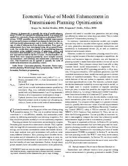
1ImprovedTransmission Planning ModelsQingyu Xu1Benjamin F Hobbs11Whiting School ofEngineeringJohns Hopkins UniversityBaltimoreUSAbhobbsjhueduAbstractA framework to quantify the value of model enhance. Mike Brewer. Programme Director, Direct Tax and Welfare team. Institute for Fiscal Studies, London, UK. © Institute for Fiscal Studies . What is . TAXBEN?. A static tax and benefit micro-simulation model of taxes on personal incomes, local taxes, expenditure taxes, and entitlement to benefits and tax credits that operates on large-scale, representative, household surveys. In collaboration with:. Elizabeth Whitaker, Erica Briscoe, Ethan . Trewhitt. , . Georgia Tech. Kevin Murphy, Frank Ritter, John . Horgan. , Penn State. Caroline Kennedy-Pipe, . Univ. of Hull. Presented to:. A Discussion with the . RAC. Trac-Compatible Vendor Community. Elizabeth Baskett, Senior Associate Director, Policy, AHA. Katie Christensen, PCS, AHA RACTrac Contractor. April 20, 2011. Agenda . Thanks for Making . Lab 2 - . Equations. Tomorrow - Tue 3-5 or 7-9 PM - SN 4117. Assignment 2 – Data Equations. Due Wednesday. Data = Model + Residual. Chapter 5. Data Equations. Data = Model + Residual. Data = Model + Residual. stage model quantifying the performances at characterize a age-group but a course of different stages the development scales which researched. Among the widely used They have study of normal two years January 1, 2017. Vision. Hearing Aid. Dental. #. Benefit Enhancements 2017. Single In-network Providers, offering . Quality Service. at . Great Value. High-quality Dental, Vision and Hearing aid care at an affordable cost—and in some cases at no cost—if members select an in-network provider . March 2014. Vision Website Enhancements Coming Soon. The member’s online experience is being enhanced with the launch of Vision Administration System. Enhancements include:. Single sign on from myuhc.com. Neil Townsend. 30 January 2017. Context. 2012-14 Evaluating 10 yearly population Census versus annual 4% sample survey. Cost benefit one of important factors in decision. Survey . option cheaper . but what about . Cory Koedel. Shawn Ni. Michael Podgursky. The Policy Event. Between 1995 and 1999, the average annual nominal return to the DJA was 25 percent.. 200 percent cumulative growth over a 5-year period.. These abnormally high returns improved funding ratios for state pension systems; many systems were reporting actuarial surpluses by the late 1990s.. WCOSS Science Quarterly Briefing. Brian Cosgrove (Office of Water Prediction). David Gochis (National Center for Atmospheric Research). Version 1.1 will be the direct follow-on to NWM version 1.0. Target Dates. Jim Waters, President, Bluegrass Institute. Aaron Ammerman, Investment Analyst*. William F. Smith, MD, Systems Analyst. *Bluegrass Institute Board Member. 2. Actuarial Funding of Benefits. YEAR. BENEFIT FACTOR. 2. O Production in the Gulf of Mexico. Presenter: Fiona(Xuejiao) Zhang. Advisors: Mike . Griffin. . Mitchell . Small. Overview. Introduction. Model development. Results and discussion. 1 Abstract — ments (VOME) in transmission planning model s is pro posed and applied to a case study of large - scale long - term planning of WECC system. VOME quantifies the probability - weig REMI Missouri Economic Model The REMI Missouri Regional Economic Model is used by the Missouri Department of Economic Development DED to forecast economic and policy impacts statewide and across R