Introduction to Hypothesis Testing - PDF document

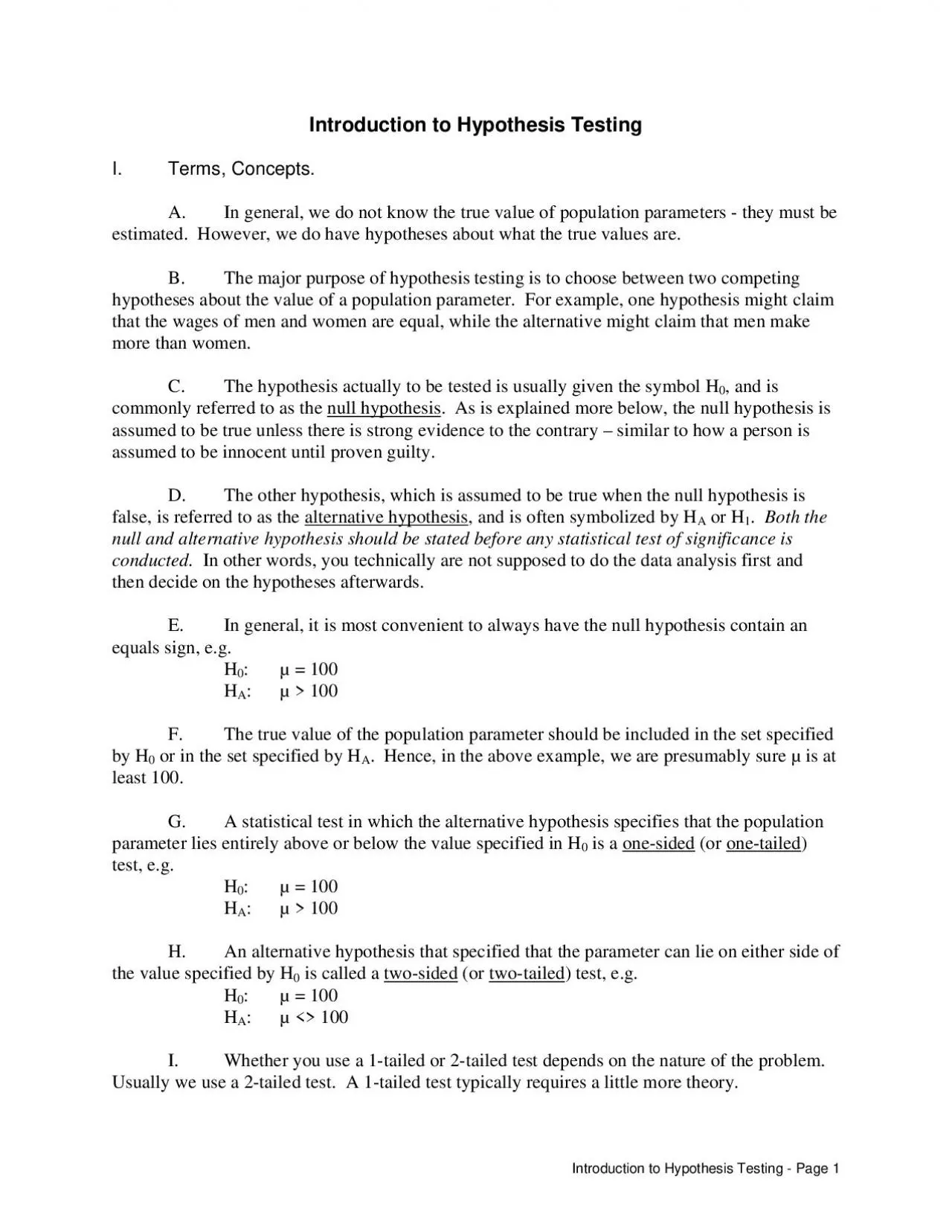
Introduction to Hypothesis Testing I. Terms, Concepts. A. In general, we do not know the true value of population parameters - they must be estimated. However, we do have hypotheses about what the true values are. B. The major purpose of hypothesis testing is to choose between two comp 0 , and is commonly referred to as the null hypothesis . As is explained more below, the null hypothesis is assumed to be true unless there is strong evidence to the contrary – similar to how a person is assumed to be innocent until proven guilty. D. The other hypothesis, which is assumed to be true when the null hypothesis is H 0 : µ = 100 H A : �µ 100 F. The true value of the population

parameter should be included in the set specified by H 0 or in the set specified by H A H A : �µ 100 H. An alternative hypothesis that specified that the parameter can lie on either side of the value specified by H 0 is called a two-sided (or two-tailed ) test, e.g. H 0 For example, suppose the null hypothesis is that the wages of men and women are equal. A two-tailed alternative would simply state that the wages are not equal – implying that men could make more than women, or they could make less. A one-tailed alternative would be that men make more than women. The latter is a stronger statement and requires more theory, in that not only are you claiming that there is a difference, y

ou are stating what direction the difference is in. J. In practice, a 1-tailed test such as H 0 : µ = 100 H A : �µ 100 is tested the same way as H 0 : µ 100 H A : �µ 100 For exam�ple, if we conclude that µ 100, we mu��st also conclude that µ 90, µ 80, etc. II. The decision problem. A. How do we choose between H 0 and H A ? The standard procedure is to assume H 0 is true - just as we presume innocent until proven guilty. Using probability theory, we try to determine whether there is sufficient evidence to declare H 0 false. B. We reject H 0 only when the chance is small that H 0 is true. Since our decisions are based on probabilit

y rather than certainty, we can make errors. C. Type I error - We reject the null hypothesis when the null is true. The probability of Type I error = . Put another way, = Probability of Type I error = P(rejecting H 0 | H 0 is true) Typical values chosen for are .05 or .01. So, for example, if = .05, there is a 5% chance that, when the null hypothesis is true, we will erroneously reject it. D. Type II error - we accept the null hypothesis when it is not true. Probability of Type II error = ß . Put another way, ß = Probability of Type II error = P(accepting H 0 | H 0 is false) E. EXAMPLES of type I and type II error: H 0 : µ = 100 H A : �µ Introduction

to Hypothesis Testing - Page 2 Suppose µ really does equal 100. But, suppose the researcher accepts H A instead. A type I error has occurred. Or, suppose µ = 105 - but the researcher accepts H 0 . A type II error has occurred. The following tables from Harnett help to illustrate the different types of error. F. and ß are not independent of each other - as one increases, the other decreases. However, increases in N cause both to decrease, since sampling error is reduced. G. In this class, we will primarily focus on Type I error. But, you should be aware that Type II error is also important. A small sample size, for example, might lead to frequent Type II errors, i.e. it could be that

your (alternative) hypotheses are right, but because your sample is so small, you fail to reject the null even though you should. III. Hypothesis testing procedures. The following 5 steps are followed when testing hypotheses. 1. Specify H 0 and H A - the null and alternative hypotheses . Examples: (a) H 0 : E(X) = 10 H A : �E(X) (b) H 0 : E(X) = 10 H A : E(X) (c) H 0 : E(X) = 10 H A : �E(X) 10 Note that, in example (a), the alternative values for E(X) can be either above or below the value specified in H 0 . Hence, a two-tailed test is called for - that is, values for H A lie in both the upper and lower halves of the normal distribution. In example (b), th

e alternative values are below those specified in H 0 , while in example (c) the alternative values are above those specified in H 0 . Hence, for (b) and (c), a one-tailed test is called for. Introduction to Hypothesis Testing - Page 3 When working with binomially distributed variables, it is often common to use the proportion of successes, p, in the hypotheses. So, for example, if X has a binomial distribution and N = 20, the above hypotheses are equivalent to: (a) H 0 : p = .5 H A : �p (b) H 0 : p = .5 H A : p (c) H 0 : p = .5 H A : �p .5 2. Determine the appropriate test statistic . A test statistic is a random variable used to determine how close a specific samp

le result falls to one of the hypotheses being tested. That is, the test statistic tells us, if H 0 is true, how likely it is that we would obtain the given sample result. Often, a Z score is used as the test statistic. For example, when using the normal approximation to the binomial distribution, an appropriate test statistic is qNpNp - .5 successesof # =z 000 where p 0 and q 0 are the probabilities of success and failure as implied or stated in the null hypothesis. When the Null hypothesis is true, Z has a N(0,1) distribution. Note that, since X is not actually continuous, it is sometimes argued that a correction for continuity should be applied. To do this, add .5 to x when x 0 , and subtra

ct .5 from� x when x Np 0 . Note that the correction for continuity reduces the magnitude of z. That is, failing to correct for continuity will result in a z-score that is too high. In practice, especially when N is large, the correction for continuity tends to get ignored, but for small N or borderline cases the correction can be important. Warning (added September 2004): As was noted earlier, the correction for continuity can sometimes make things worse rather than better. Especially if it is a close decision, it is best to use a computer program that can make a more exact calculation, such as Stata can with its bitest and bitesti routines. We will discuss this more later. Intuitively,

what we are doing is comparing what we actually observed with what the null hypotheses predicted would happen; that is, # of successes is the observed empirical result, i.e. what actually happened, while Np 0 is the result that was predicted by the null hypothesis. Now, we know that, because of sampling variability, these numbers will probably not be exactly equal; e.g. the null hypotheses might have predicted 15 successes and we actually got 17. But, if the difference between what was observed and what was predicted gets to be too great, we will conclude that the values specified in the null hypotheses are probably not correct and hence the null should be rejected. Introduction to Hypothesis Testing - P