PDF-AMERICAN METEOROLOGICAL SOCIETY

Author : karlyn-bohler | Published Date : 2016-05-24

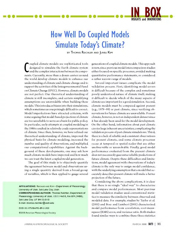
303 AMERICAN METEOROLOGICAL SOCIETY e nal model performance index was formed by taking the mean over all climate variables Table 1 and one model using equal weights mvm

Presentation Embed Code

Download Presentation

Download Presentation The PPT/PDF document "AMERICAN METEOROLOGICAL SOCIETY" is the property of its rightful owner. Permission is granted to download and print the materials on this website for personal, non-commercial use only, and to display it on your personal computer provided you do not modify the materials and that you retain all copyright notices contained in the materials. By downloading content from our website, you accept the terms of this agreement.

AMERICAN METEOROLOGICAL SOCIETY: Transcript

303 AMERICAN METEOROLOGICAL SOCIETY e nal model performance index was formed by taking the mean over all climate variables Table 1 and one model using equal weights mvm 3The final step comb. brPage 1br Indian Meteorological Society Local Chapter AHMEDABAD CHAPTER BANGALORE CHAPTER BHOPAL CHAPTER BHUBANESWAR CHAPTER CHANDIGARH CHAPTER CHENNAI CHAPTER COCHIN CHAPTER DEHRADUN CHAPTER D 1. MOTION. That the Council approves the continuation of: . Committee on Patents and Related Matters (CP&RM. ), . subject . to the concurrence by the Board of . Directors. Committee on Technician Affairs (CTA) . 25-27August 2015. Addis Ababa, Ethiopia . Reports from Strengthening National Climate Information/ . Early Warning System (CI/EWS) Projects. Ethiopia. Ababu Anage. National Climate Change Specialist. PHILLIP OKELLO OCHIENG. Meteorologist/Research Scientist. Geosciences and Tsunami Information Services. Kenya Meteorological Service. Email: pokello@meteo.go.ke. CAP Implementation . in Kenya. KENYA. . M. eteorological. . D. epartment. . (. JMD. ). Mohammad . Samawi. Deputy Director General. Jordan Meteorological Department. . JMD. Training Workshop for National Meteorological and Hydrological Services (NMHSs) on Designing Socio-Economic Benefits Studies of Meteorological/Hydrological Services and Products for Members of Regional Association VI (Europe). Value Chains. Jeffrey K .Lazo, PhD. Director – Societal Impacts Program. National Center for Atmospheric Research. Zagreb, Croatia. Monday, 29 June 2015. 1600-1630. NMHS Mission . and Functions. UK . PM. 2.5. . air quality inferred from a multi-model analysis of meteorological modes. Loretta J. Mickley. Co-Is:. Amos P.K.A. Tai. . and Daniel J. Jacob. School of Engineering and Applied Sciences. Harvard University. . STATUS REPORT . Lamin. Mai . Touray. , Project Director. Ousman. . Jarjusey. , Project Coordinator. Bubu Pateh Jallow, Chief Technical Adviser. Department of Water Resources. 7 Marina Parade, Banjul. ACS GCI . Pharmaceutical Roundtable’s. Convergent PMI* Calculator. *Process Mass Intensity. ACS GCI . Pharmaceutical . Roundtable. Mission. : . To . catalyze the implementation of . green chemistry . and . Dispersion . Support. Walt Schalk. Air Resources Laboratory. June 21, 2016. The Research Flow. ARL Science Review, June 21-23, 2016. 2. Research. Application. R2A. Research To Application. The Research Flow. Integrated Meteorological Information H. Sudarshan SIP/2012/ASBU/Nairobi -WP/18 Workshop on preparations for ANConf/12 − ASBU methodology (Nairobi, 13-17 August 2012) 2 Outline Does MET matter to ATM efficiency? ZAMBIA. Mukufute. M. . Mukelabai. Introduction. Progress and Key Successes. Concerns, Challenges, Opportunities. Last Mile. Meteorological Monitoring Equipment and Systems. 28 Automatic Weather Stations – ordered and delivered to Zambia Meteorological Department. Geodynamics (ZAMG) Hohe Warte 38 A - 1190 - Vienna AUSTRIA Royal Meteorological Institute of Belgium (RMI) Avenue Circulaire 3, B 1180 - Brussels BELGIUM Meteorological and Hydrological Service of National Institute of Meteorology (INMET), Brazil. Advisor to the Director and Head of International Affairs. World Meteorological Organization. 21 July 2022, Cartagena de . Indias. , Colombia. HIGH-LEVEL REGIONAL FORUM OF THE.

Download Document

Here is the link to download the presentation.
"AMERICAN METEOROLOGICAL SOCIETY"The content belongs to its owner. You may download and print it for personal use, without modification, and keep all copyright notices. By downloading, you agree to these terms.