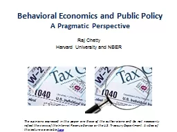
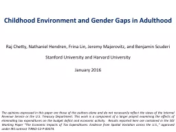
Hendren Harvard Patrick Kline UCBerkeley Emmanuel Saez UCBerkeley Nicholas Turner Office of Tax Analysis Is the United States Still a Land of Opportunity Recent Trends in Intergenerational Mobility ID: 723828
Download Presentation The PPT/PDF document "Raj Chetty , Harvard Nathaniel" is the property of its rightful owner. Permission is granted to download and print the materials on this web site for personal, non-commercial use only, and to display it on your personal computer provided you do not modify the materials and that you retain all copyright notices contained in the materials. By downloading content from our website, you accept the terms of this agreement.
Slide1
Raj
Chetty, HarvardNathaniel Hendren, HarvardPatrick Kline, UC-BerkeleyEmmanuel Saez, UC-BerkeleyNicholas Turner, Office of Tax Analysis
Is the United States Still a Land of Opportunity?Recent Trends in Intergenerational Mobility
The opinions expressed in this paper are those of the authors alone and do not necessarily reflect the views of the Internal Revenue Service or the U.S. Treasury
Department. This
work is a component of a larger project examining the effects of eliminating tax expenditures on the budget deficit and economic activity
. Certain results
reported
here are taken from the
SOI
Working
Paper “The Economic Impacts of Tax Expenditures: Evidence from Spatial Variation
across the
U.S.,” approved under
IRS contract TIRNO-12-P-00374.Slide2
Growing public perception that intergenerational mobility has declined in the United StatesVast literature has investigated whether this is true empirically [e.g., Aaronson and Mazumder 2008, Lee and Solon 2009, Auten, Gee, and Turner 2013]Results debated partly due to limitations in data [Black and Devereux 2011]
IntroductionSlide3
We analyze trends in mobility for 1971-1993 birth cohorts using administrative data on more than 50 million children and their parentsTwo main empirical resultsRelationship between parent and child percentile ranks (i.e. the copula) is extremely stableChance of moving from bottom to top fifth of income distribution no lower for children entering labor market today than in the 1970sInequality increased in this sample, consistent with prior workConsequences of the “birth lottery” – the parents to whom a child is born – are larger today than in the past
This PaperSlide4
We use de-identified data from federal income tax returnsIncludes non-filers via information forms (e.g. W-2’s)DataSlide5
Parent(s) defined as first person(s) who claim child as a dependent
Can reliably link children to parents up to age 16, after which some children leave the houseWe link approximately 90% of children to parents overallLinking Children to ParentsSlide6
Population tax records starting in 1996Data on children and parents for the 1980-1993 birth cohorts40 million children, age 20-31 in 2011Statistics of Income 0.1% Stratified Random Samples 1987-1997Data on children and parents for the 1971-1982 birth cohorts
Two SamplesSlide7
Parent Income: mean pre-tax household income (AGI+SSDI)Child Income: mean pre-tax household income ages 26 or 29-30For non-filers, use W-2 wage earnings + SSDI + UI incomeIf no 1040 and no W-2, code income as 0These household level definitions capture total resources in the householdResults robust to using individual-level income measures
Income DefinitionsSlide8
Measuring Intergenerational MobilitySlide9
Previous literature has measured mobility using various statisticsLog-log intergenerational elasticity Rank-rank correlationsTransition matricesEach of these could potentially exhibit different time trendsBegin by formalizing how we measure mobility
Measuring MobilitySlide10
We decompose joint distribution of parent and child income into two componentsJoint distribution of parent and child percentile ranks (i.e., copula of distribution)Marginal distributions of parent and child incomeMarginal distributions determine inequality within generationsCopula is the key determinant of mobility across generationsRank-rank and transition matrix depend purely on copulaLog-log IGE combines copula and marginal distributions
Measuring MobilitySlide11
We study all three measures, but use a rank-rank specification as our primary measureRank children based on their incomes relative to other children in same birth cohortRank parents of these children based on their incomes relative to other parents in this sampleIn our companion paper on geography of mobility, we show that rank-rank has statistical advantages over other measures
Rank-Rank SpecificationSlide12
20
30
40
50
60
70
0
10
20
30
40
50
60
70
80
90
100
Mean Child Income Rank
Parent Income Rank
Mean Child Percentile Rank vs. Parent Percentile Rank
Rank-Rank Slope (U.S)
= 0.341
(0.0003)Slide13
Literature has emphasized two sources of potential bias in estimates of intergenerational elasticitiesLifecycle bias: measuring earnings too early or too lateAttenuation bias: measuring transitory rather than permanent income
Lifecycle and Attenuation BiasSlide14
0
0.1
0.2
0.3
0.4
22
25
28
31
34
37
40
Age at which Child’s Income is Measured
Population
Rank-Rank Slope
Lifecycle Bias: Intergenerational Income Correlation
by Age at Which Child’s Income is MeasuredSlide15
0
0.1
0.2
0.3
0.4
22
25
28
31
34
37
40
Age at which Child’s Income is Measured
Population
SOI 0.1% Random Sample
Rank-Rank Slope
Lifecycle Bias: Intergenerational Income Correlation
by Age at Which Child’s Income is MeasuredSlide16
1
4
7
10
13
16
Rank-Rank Slope
Years Used to Compute Mean Parent Income
Attenuation Bias: Rank-Rank Slopes
by Number of Years Used to Measure Parent Income
0
0.1
0.2
0.3
0.4Slide17
Time TrendsSlide18
30
40
50
60
70
0
20
40
60
80
100
1971-74
71-74 Slope = 0.299
(0.009)
Child Income Rank vs. Parent Income Rank by Birth Cohort
Parent Income Rank
Mean Child Income
RankSlide19
30
40
50
60
70
0
20
40
60
80
100
1971-74
1975-78
71-74 Slope = 0.299
(0.009)
75-78
Slope
= 0.291
(0.007)
Child Income Rank vs. Parent Income Rank by Birth Cohort
Parent Income Rank
Mean Child Income
RankSlide20
30
40
50
60
70
0
20
40
60
80
100
Parent Income Rank
1971-74
1975-78
1979-82
71-74 Slope = 0.299
(0.009)
75-78
Slope
= 0.291
(0.007)
79-82
Slope = 0.313
(0.008)
Child Income Rank vs. Parent Income Rank by Birth Cohort
Mean Child Income
RankSlide21
0
0.2
0.4
0.6
0.8
1971
1974
1977
1980
1983
1986
1989
1992
Child's Birth Cohort
Income Rank-Rank
(Child Age 30)
Intergenerational Mobility Estimates for the 1971-1993 Birth Cohorts
Rank-Rank SlopeSlide22
0
0.2
0.4
0.6
0.8
1971
1974
1977
1980
1983
1986
1989
1992
Child's Birth Cohort
Income Rank-Rank
(Child Age 30; SOI Sample)
Income Rank-Rank
(Child Age 26; Pop. Sample)
Intergenerational Mobility Estimates for the 1971-1993 Birth Cohorts
Rank-Rank SlopeSlide23
For younger cohorts, it is too early to measure earnings But we can measure college attendance, which is a strong predictor of earningsMoreover, college-income gradient is highly correlated with income rank-rank slope across areas of the U.S. [Chetty et al. 2014]Define college attendance as attending when age 19Results similar if attendance measured at later ages
College GradientSlide24
1984-87
Parent Income Rank
20%
40%
60%
80%
100%
0
20
40
60
80
100
84-87
Slope = 0.745
(0.008)
Percent in College at 19
College Attendance Rates vs. Parent Income Rank by CohortSlide25
1984-87
1988-90
Parent Income Rank
20%
40%
60%
80%
100%
0
20
40
60
80
100
84-87
Slope = 0.745
(0.008)
88-90
Slope
= 0.742
(0.010)
Percent in College at 19
College Attendance Rates vs. Parent Income Rank by CohortSlide26
1984-87
1988-90
1991-93
Parent Income Rank
20%
40%
60%
80%
100%
0
20
40
60
80
100
84-87
Slope = 0.745
(0.008)
88-90
Slope
= 0.742
(0.010)
91-93
Slope = 0.705
(0.013)
Percent in College at 19
College Attendance Rates vs. Parent Income Rank by CohortSlide27
0
0.2
0.4
0.6
0.8
1971
1974
1977
1980
1983
1986
1989
1992
Child's Birth Cohort
Intergenerational Mobility Estimates for the 1971-1993 Birth Cohorts
Income Rank-Rank
(Child Age 30; SOI Sample)
College-Income Gradient
(Child Age 19; Pop. Sample)
Income Rank-Rank
(Child Age 26; Pop.
Sample
)
Rank-Rank SlopeSlide28
0
0.2
0.4
0.6
0.8
Rank-Rank Slope
1971
1974
1977
1980
1983
1986
1989
1992
Child's Birth Cohort
Intergenerational Mobility Estimates for the 1971-1993 Birth Cohorts
Forecast Based on Age
26
Income
and College Attendance
Income Rank-Rank
(Child Age 30; SOI Sample)
College-Income Gradient
(Child Age 19; Pop. Sample)
Income Rank-Rank
(Child Age 26; Pop.
Sample
)Slide29
Can obtain a richer prediction of earnings by using information on which college student attendedDefine “college quality” as mean earnings at age 31 of children born in 1979-80 based on the college they attended at age 20College QualitySlide30
1984-87
1988-90
1991-93
Parent Income Rank
30
40
50
60
70
80
0
20
40
60
80
100
Mean College Quality Rank
84-87
Coll.
Qual
Gradient
(P75-P25)
= 0.191
88-90
Coll.
Qual
Gradient (P75-P25)
= 0.192
91-93
Coll.
Qual
Gradient (P75-P25)
= 0.181
College Quality Rank vs. Parent Income Rank by CohortSlide31
Trends in College Attendance vs. College Quality Gradients
0
.2
.4
.6
.8
0
.05
.1
.15
.2
1984
1986
1988
1990
1992
1994
College Quality Gradient (P75-P25)
College Attendance Gradient
College Quality
College Attendance
Child’s Birth CohortSlide32
Mobility also stable using other statisticsEx: fraction of children who reach the top quintile Quintile Transition ProbabilitiesSlide33
0%
10%
20%
30%
40%
1971
1974
1977
1980
1983
1986
Child's Birth Cohort
Parent Quintile
Probability of Reaching Top Quintile by Birth Cohort
Q1
Q3
Q5
Probability Child in Top Fifth of Income DistributionSlide34
Substantial heterogeneity in mobility across areas[Chetty, Hendren, Kline, Saez 2014]Do these differences persist over time?Regional HeterogeneitySlide35
0
0.2
0.4
0.6
0.8
Rank-Rank Slope
1980
1982
1984
1986
1988
1990
1992
Pacific
Mountain
New England
East South Central
Child's Birth Cohort
Intergenerational Mobility Estimates by
Parent’s Census Division
College Attendance
Age 26 Income RankSlide36
Rank-based mobility is not declining in the U.S. as a wholeCombined with evidence from Lee and Solon (2009), mobility appears to be roughly stable over past half centuryBut mobility is (and has consistently been) low in the U.S. relative to most other developed countries (Corak 2013)Increased inequality consequences of the “birth lottery” largerLow mobility matters more today than in the past
DiscussionSlide37
Results may be surprising given negative correlation between mobility and inequality in cross-section [Corak 2013]Based on “Great Gatsby Curve,” one would predict that mobility should have fallen by 20% [Krueger 2012]One explanation: much of the increase in inequality is driven by extreme upper tail (top 1%)But top 1% income shares are not strongly correlated with mobility across countries or across areas within the U.S. [Chetty et al. 2014]Predicted increase in rank-rank slope based on bottom 99% Gini coefficient (“middle class inequality”) is only 0.3 to 0.32
DiscussionSlide38
Key open question: why do some parts of the U.S. have persistently low rates of intergenerational mobility? Mobility statistics by birth cohort by commuting zone available on project website (www.equality-of-opportunity.org)Future ResearchSlide39
Download Data on Social Mobility
www.equality-of-opportunity.org/dataSlide40
Appendix FiguresSlide41
0
0.2
0.4
0.6
0.8
3
6
9
12
15
18
Age of Child when Parent Income is Measured
Slope of College Attendance Gradient by
Age of Child when Parent Income is Measured
College Attendance GradientSlide42
Years Used to Compute Mean Child Income
1
2
3
4
5
0
0.1
0.2
0.3
0.4
Rank-Rank Slope
Attenuation Bias:
Rank-Rank Slopes by
Number of Years Used to Measure Child IncomeSlide43
Age
at which Parent Income is Measured
0
0.1
0.2
0.3
0.4
41
43
45
47
49
51
53
55
Rank-Rank Slope
Rank-Rank Slope by Age at which Parent Income is MeasuredSlide44
0
0.2
0.4
0.6
0.8
1981
1983
1985
1987
1989
1991
1993
Child’s Birth Cohort
Before Age 19
Before Age 20
Before Age 22
Before Age 25
Slope of Coll. Attendance by Par. Income Gradient
Robustness of College Attendance Gradient by
Age at which College Attendance is Measured