Stock returns macroeconomic variables - PDF document

1 Stock returns, macroeconomic variables
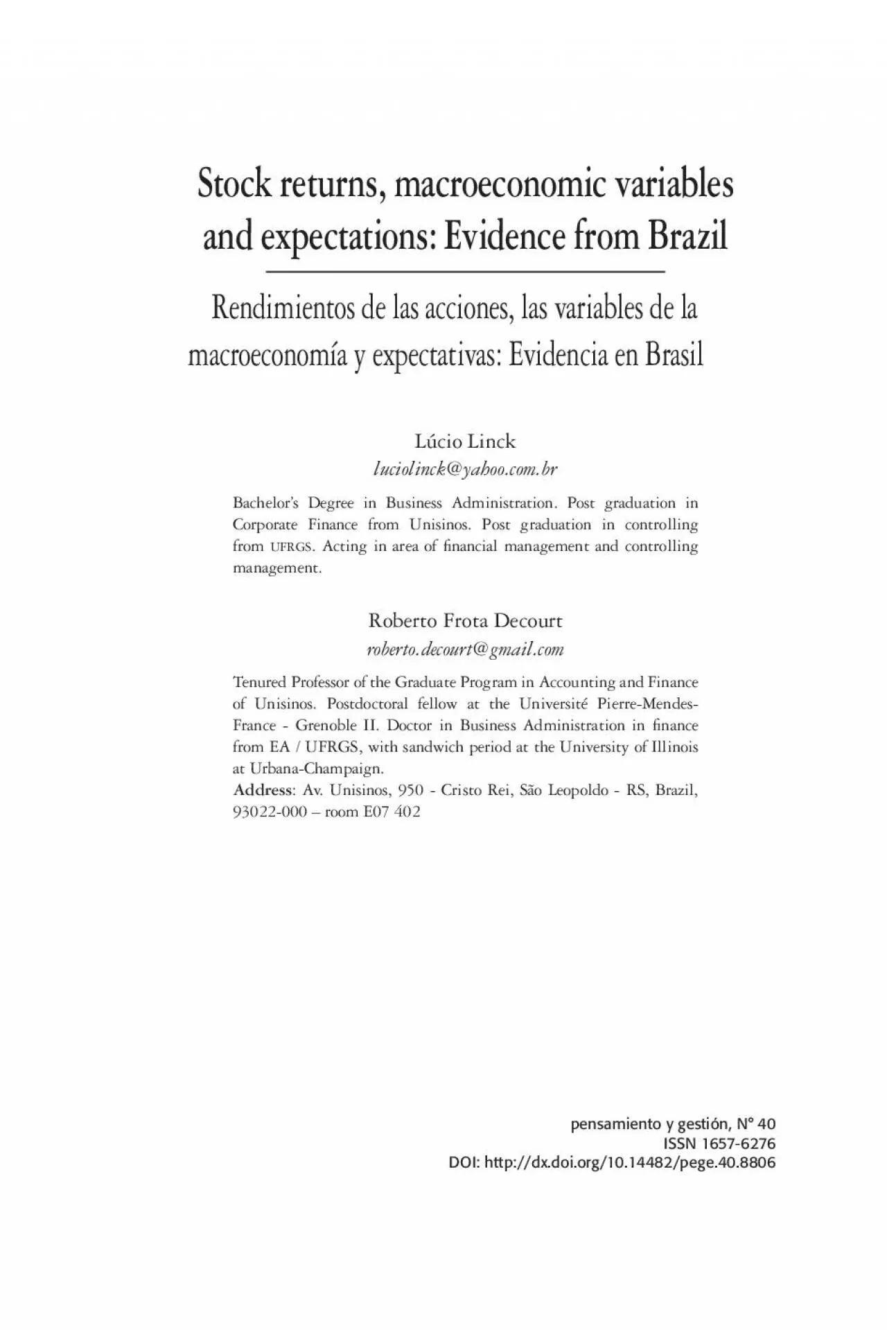
Stock returns, macroeconomic variables and expectations: Evidence from Brazil Rendimientos de las acciones, las variables de la macroeconomía y expectativas: Evidencia en Brasil Lúcio Linck luciolinck@yahoo.com.br Bachelor’s Degree in Business Administration. Post graduation in Corporate Finance from Unisinos. Post graduation in controlling from UFRGS . Acting in area of nancial management and controlling management. Roberto Frota Decourt roberto.decourt@gmail.com Tenured Professor of the Graduate Program in Accounting and Finance of Unisinos. Postdoctoral fellow at the Université Pierre-Mendes- France - Grenoble II. Doctor in Business Administration in nance from EA / UFRGS, with sandwich period at the University of Illinois at Urbana-Champaign. Address : Av. Unisinos, 950 - Cristo Rei, São Leopoldo - RS, Brazil, 93022-000 – room E07 402 pensamiento y gestión, N° 40 ISSN 1657-6276 DOI: http://dx.doi.org/10.14482/pege.40.8806 Abstract There is not general support to explain the correlation among the ma - croeconomic variables and share returns in different countries and time. The unique characteristics of the Brazilian economy have changed deeply over the last years, thus the purpose of this study is to explore the correla - tion among the macroeconomic variables and share returns in Brazil from 2000 to 2010. The study investigates the causality relationships among real stock returns, basic interest rates, GDP , ination and the market expec - tation of future behavior of these macroeconomic variables. The method used to nd the correlation among the variables studied was the Ste - pwise Multiple Regression. The results show that basic interest rates and GDP affect the stock returns, however ination and market expectation of future behavior of these macroeconomic variables affect stock returns i

2 nsignicantly. Keywords: stock retu
nsignicantly. Keywords: stock returns; capital Market; macroeconomics variables. Resumen La relación entre las variables macroeconómicas y los rendimientos de las acciones tiene resultados diferentes dependiendo de la ubicación y el tiem - po que se estudiaron. Como Brasil tiene en los últimos años características peculiares, este estudio tiene como objetivo determinar el impacto de las variables y las expectativas sobre el rendimiento de las acciones entre 2000 y 2010. Las tasas de inación macroeconómicas fueron probados ( IPCA y IGP-M ), meta para la tasa Selic y la variación del PIB actual y también la expectativa del mercado para el futuro. El método utilizado para identicar la relación entre las variables y el retorno de las acciones se basó en la esti - mación de regresión múltiple por pasos. Se identicó que la tasa de interés y el PIB afectan rendimientos de las acciones. La inación y las expectativas del comportamiento futuro de las variables no mostraron correlación signi - cativa con la rentabilidad de las acciones. Palabras clave: rendimientos de las acciones; los mercados de capitales; Variables macroecômicas. Fecha de recepción: 15 de febrero de 2016 Fecha de aceptación: 17 de marzo de 2016 93 pensamiento & gestión, 40. Universidad del Norte, 91-112, 2016 1. INTRODUCTIÓN Macroeconomic conditions affect the nancial results of companies be - cause their sales and margins are correlated with economic growth, in - terest rates, ination, and unemployment in the environment in which they operate. For this reason, macroeconomic indicators are widely used in the fundamentalists’ models of pricing stocks. Certain economic sec - tors are more or less sensitive to those variables, but part of a rm’s value depends not only on current performance, but also on

3 the expectation of how those macroecon
the expectation of how those macroeconomic variables will behave in the future. This expectation concerning the macroeconomic variables’ performance in the future is an important point in asset pricing because, for an inves - tor, the important thing to consider when evaluating an investment is how much will potentially be paid in the future balanced against the risk assumed at the time of application (Fama, 1981). Past performances will not necessarily be repeated in the future. This is why we believe that stock performance is correlated not only with macroeconomic variables (Fama, 1981; Bhattacharya & Mukherjee, 2006; Flannery & Protopapadakis, 2002), but also with the expectation of how those variables will behave in the future. A strong and efcient capital market gives companies access to investors’ resources to invest in their projects; therefore, an efcient capital mar - ket is essential for the economic development of a country, as it allows companies to access investors’ resources to grow and cultivate a stronger economy. Brazil has a recent history of hyperination, which was nally contro - lled in 1994, but despite that apparent stability, the ination rate is still considered high compared to most other countries. Since 1994, the prime rate, one of the main instruments for controlling ination in Bra - zil, has been one of the world’s largest, and economic growth uctuated dramatically during this period, being above the world average in some years and then dropping below that average in others. Still, during this period, the Brazilian capital market showed signicant progress, likely as 94 pensamiento & gestión, 40. Universidad del Norte, 91-112, 2016 a consequence of higher economic stability and the evolution of corporate governance practices in the country. Terra (200

4 6) examined the effects of stocks in 14
6) examined the effects of stocks in 14 different countries and found that it is not possible to nd an appropriate universal explanation to connect ination and stock returns. Thus, these characteristics of the Brazilian market motivated us to conduct this study. A more compre - hensive understanding of the inuence of macroeconomic indicators and their expectations of the Brazilian stock market may be useful to regula - tors, investors, and researchers. Contrary to what is expected, the expectations of macroeconomic va - riables were not relevant in the evaluation of the shares, and only the interest and economic growth were statistically signicant in our model. This article presents a brief theory revision on the subject in Chapter 2, the method is outlined in Chapter 3, the results can be found in Chapter 4, and nal remarks compose Chapter 5. 2. THEORETICAL REVIEW Bodie (1976) tested the efciency of investment in shares as a mechanism of protection against ination; annual and monthly data over a period of 20 years (1953-1972) was studied, but to the author’s surprise, the return of the shares was inversely correlated with ination. Fama (1981) argued that the inverse relationship between ination and stock returns is the result of a spurious relationship, because there is also an inverse correlation between ination and future economic activity and stock prices tend to anticipate future economic activity. Shares had fallen during times of high ination, because overall economic activity, in the long run, is impaired by ination. Cutler, Poterba, and Summers (1989) analyzed the correlation between stock returns and industrial production growth in the period from 1926 to 1986. Using the full sample, a signicant correlation between the two variables was found. However, consid

5 ering only the period between 1946 and
ering only the period between 1946 and 1985, industrial output growth and stock returns did not present a 95 pensamiento & gestión, 40. Universidad del Norte, 91-112, 2016 signicant correlation. The authors tested the hypothesis that ination and interest rates affect long-term stock returns, but were unable to nd support for this hypothesis. Boyd, Jagannathan, and Hu (2005) analyzed the effect of making announ - cements regarding macroeconomic variables in different economic periods. The authors analyzed the effect of tax advertisements on unexpected unem - ployment by the stock market and various effects on the S&P 500 for the period of 1948 to 1995. The study concluded that the unexpected hikes in unemployment taxes added value to the stocks during periods of economic growth, but undervalued their shares in periods of economic contraction. Fama (1990) argued that the stocks reect the future cash ow of the companies; in this way, variations in stock prices could predict future macroeconomic variables. Gay (2008) examined the effects of macroeconomic variables of stock prices in emerging markets. The study was conducted in Brazil, China, India, and Russia; it tested the impact of changes in exchange rates and the price of oil share worth. No signicant results were found, which led the author to conclude that in emerging markets, domestic factors have a greater inuence on stock returns than external factors, such as was evidenced in the study. In Brazil, Magalhães (1982) studied the relationship between stock re - turns and expected and unexpected ination between 1972 and 1980. Expected ination was not associated with stock returns, but the author did nd a positive correlation for unexpected returns. Sanvicente, Adrangi, and Chatrath (2002) also studied the relationship between inat

6 ion and stock returns in Brazil and foun
ion and stock returns in Brazil and found a negative co - rrelation between the variables in a study conducted in the early years of hyperination and the stabilization of the Plano Real (1986 to 1997), which correlated macroeconomic variables with the Bovespa Index. Terra (2006) examined the effect of ination on stock returns in Brazil and 13 other countries, with a sample composed of seven countries in 96 pensamiento & gestión, 40. Universidad del Norte, 91-112, 2016 Latin America and seven industrialized countries. The period covered was not the same for each country, the longest being the one measured in Canada (1970-2000) and the shortest from the sample in Peru (1993- 1999). For Brazil, the period from 1982 to 1999 was considered. The author suggested that in Brazil there were articial stock returns because ina - tion caused the valuation of depreciation and inventories that increased the taxable income of the companies at the expense of the actual return in stocks. Caselani and Eid (2008) analyzed the effect of macroeconomic variables on stock prices. To do this, they used composite returns from 35 compa - nies on the Bovespa Index between 1995 and 2003. The authors found a positive relationship between real interest rates and stock returns, but a negative relationship between industrial production and stock returns. Method To identify the inuence of macroeconomic variables on stock price, the monthly variations of the Bovespa index during the period of 2000 to 2010 is the dependent variable; the macroeconomic indices of ination ( IPCA and IGP-M ), SELIC target rates, and the change in GDP are the inde - pendent variables. Macroeconomic data was represented by facts or in the actual and selected data, as presented in Table 1. Table 1 . Data Selection of Macroeconomic Facts Variable Data selection P

7 eriod GDP Change in quarter compared wit
eriod GDP Change in quarter compared with the same quarter one year before. Third period - the publication of data. IGP-M Last 12 months. Subsequent period. IPCA Last 12 months. Subsequent period. Selic target Monthly Within the same period. 97 pensamiento & gestión, 40. Universidad del Norte, 91-112, 2016 As GDP data is accumulated quarterly, however this research works with monthly variations, thus, for the three months of each quarter was used the same variation in the quarterly GDP . To complete the independent variables, the study also utilized the same systematic indexes, this time represented by the market expectations from the Focus report from the Central Bank of Brazil. In Table 2, the method of how this data was se - lected is explained. Table 2 . Data Selection of Macroeconomic Expectations Variable Data selection Period GDP-E Expectations for the year. Median of all expectations of the period (month). IGP-M-E Expectations for the year. Median of all expectations of the period (month). IPCA-E Expectations for the year. Median of all expectations of the period (month). Selic target-E Expectations for the end of the year. Median of all expectations of the period (month). The sample of this study considers the ratio between the number of ob - servations in the sample and independent variables, 16.5 to 1, i.e. for each independent variable (macroeconomic), there are 16 observations in the sample, totaling 132 data points to be observed. Hair et al. (2009) ar - gued that this ratio should be at least 5 to 1, while a desired level would be between 15 and 20 observations for each variable. At the end of each month, from 2000 to 2010, the closing value of the Bovespa Index and IBRX -100 were gathered and subsequently proces - sed by percentage, thus representing the variable-dependent multiple regression equation. Both ratios were

8 extracted from the BM & FBOVESPA we
extracted from the BM & FBOVESPA website. The method employed for the application of multiple regressions is ba - sed on stepwise estimation, where each variable is considered for inclu - sion before the development of the equation. The independent variable 98 pensamiento & gestión, 40. Universidad del Norte, 91-112, 2016 with the largest contribution is added in the equation rst, thus selecting variables for inclusion based on their incremental contribution from the variables already in the equation. The research seeks to extend the re - gression method, applying statistical signicance tests to determine the condence of the regression coefcients over many samples. As the most appropriate form of analysis and their more reliable results, macroeconomic facts and scores of stock indices were analyzed as varia - tions of absolute indices. The method of evaluation and interpretation of data is restricted to only four macroeconomic variables, although they are separated from facts and market expectations. Analysts and investors know that the stock market is sensitive to many variables, ranging from a host of other economic indices to the disclosure of fundamentalist information. The effects of an external front, such as the impacts of international news in the Brazilian scenario, are also considered as limiting factors to research. In general, the results of this study are limited only to the variables and partially explain the impact of this information on the variation of stock prices. 3. RESULTS Initially, Ibovespa scores were collected at the end of each month during the years of 2000 to 2010. Soon after, the facts and the expectations of the Central Bank were extracted in order to determine the macroeconomic variables. Given all the available data, the macroeconomic information was composed of independent variabl

9 es to the regression equation, while va
es to the regression equation, while variation from the Bovespa index was considered the dependent variable. The preferred, most reliable and chosen way for reporting the results of the regression equation was working with the variation of all variables, whether dependent or independent. The absolute independent variables without the percentage changes are strongly correlated, which ultimately indicates the presence of multicollinearity between these variables, whe - re this is harmful to the development of the equation fact. In this case, an independent variable inuences another independent variable, which 99 pensamiento & gestión, 40. Universidad del Norte, 91-112, 2016 is not appropriate. Thus, one of the correlated variables was discarded from the research. The correlation between variables is shown in Table 3. Table 3 . Correlation matrix between the independent variables GDP IGP-M IPCA Selic target GDP-E IGP-M-E IPCA-E Selic target-E GDP 1 IGP-M 0.14 1 IPCA -0.14 0.88 1 Selic target -0.07 0.74 0.79 1 GDP-E 0.74 -0.17 -0.37 -0.31 1 IGP-M-E 0.32 0.72 0.55 0.54 0.17 1 IPCA-E -0.01 0.87 0.91 0.76 -0.25 0.77 1 Selic target-E -0.01 0.71 0.73 0.95 -0.22 0.62 0.76 1 To apply the regression procedure, changes in macroeconomic indicators were determined as factor (y) and the variation of the Bovespa index was factor (x). The independent variables, macroeconomic facts, were deter - mined in the regression table with a lag period, where the data published at a particular time was posted in the next period. Such application data is related to the reading of the market in relation to market indicators. Because the data is published with a certain lag period, the market takes the reading of the information in the subsequent period, characterizing this as the most appropriate way of performing regression calculations in the research and gett

10 ing the most accurate results. However,
ing the most accurate results. However, the ma - croeconomic market expectations were not posted in the table with a lag period, but rather in the same reporting period as the market report. Estimation of Multiple Regression Model First Variable Inclusion With the regression dened in terms of dependent and independent va - riables, the sample is considered adequate for research. The next step becomes the estimation of the regression model and the overall model t. 100 pensamiento & gestión, 40. Universidad del Norte, 91-112, 2016 The stepwise estimation procedure was used as a model to perform mul - tiple regression analysis. This procedure aims to maximize the coefcient of determination, R², through the variable with the highest partial co - rrelation, for each independent variable added to the equation. To dene the rst variable to be included in the regression model, we considered the macroeconomic indicator of the largest bivariate correlation with the monthly return of Ibovespa. Table 4 . Correlation Matrix IbovespaX1-GDPX2-IGP-MX3-IPCAX4-Selic targetX5-GDP-EX6-IGP-M-EX7-IPCA-EX8-Selic target-EIbovespaGDP0.2IGP-M-0.050.05IPCA-0.090.020.24Selic target-0.250.090.280.41GDP-E0.020.01-0.05-0.15-0.06IGP-M-E0.080.090.020.040.10.56IPCA-E-0.070.130.080.210.29-0.250.12Selic target-E-0.070.080.050.160.32-0.5-0.250.61 Table 4 shows the correlation between the independent variables and the correlation between the Bovespa and all the macroeconomic indicators. According to Table 4, we can identify that variable X4 (Meta Selic - Fact) has the highest bivariate correlation with the dependent variable Boves - pa. Thus, this is the rst variable to be added to the multiple regression equation, with an acceptable level of signicance of 0.05 for the regres - sion coefcients. The results of the regression between the variab

11 le X4 (Meta Selic - Fact) and the Boves
le X4 (Meta Selic - Fact) and the Bovespa Index are shown in Figure 1. 101 pensamiento & gestión, 40. Universidad del Norte, 91-112, 2016 Multiple R0.2483R Square0.0616Adjuste R Square0.0543Standard Error0.0762Observations130ANOVAdfSSSignificance FRegression0.04880.04888.40770.0044Residual1280.74290.0058Total1290.7917CoeficientsStandard Errort StatP-valuePartial CorrelationToleranceVIFIntercept0.01190.00671.76740.0796variable X4 (Meta Selic - Fact) -0.49650.1712-2.89960.00440.2483 Regression Statistics Collinearity Statistic Figure 1 . Results with one independent variable - X4 (Meta Selic - Fact) From the results presented in Figure 1, we can draw some conclusions from the model: • R-Multiple : the correlation coefcient for a simple regression (only one dependent variable). At this stage, it is only diagno - sing a 24.83% degree of association between Ibovespa and Meta Selic; • R-Square: Indicates the variation explained by the Bovespa in - dex variable X4-Meta Selic, which means that the interest rate explains 6.16% of the variation in the Bovespa index; • Adjusted R-squared : the coefcient with the function of mi - nimizing the equation overtting. Thus, the adjusted coefcient eliminates certain distortions in R² when the number of observa - tions in the sample is very close to the dependent variable. In the present study, this coefcient is 5.43%, not much different from the R ², which partly indicates the lack of overtting; • Standard Error : this is the square root of the sum of squared errors divided by the number of degrees of freedom, indicating an estimate of the standard deviation of the forecast errors. In our case study, this deviation was 7.61%; 102 pensamiento & gestión, 40. Universidad del Norte, 91-112, 2016 • Analysis of variance : the sum of squared errors using only t

12 he Y average to make the prediction of
he Y average to make the prediction of the dependent variable. Using the X4 variable, this error is reduced by 6.16% (0.0488/0.7917). This result indicates that by using the sample for estimation, we can demonstrate the variation six times more than by using the average, with an F ratio of 8.4077 at a signicance level of 0.044; • Analysis of Variable X4 Introduced into the Equation: a Meta Selic (fact) was considered statistically signicant for the sample (0.0044), with a regression coefcient of -0.4965; The standard error of the coefcient, estimated as the regression coef - cient, can vary in multiple samples (standard deviation of the regression coefcient), and indicated a value of 0.1712. The statistical collinearity indicator of the correlation between the inde - pendent variables (a satisfactory number should be equal or close to 1), was equal to 1, since we were only working with one variable. Out of Equation Variables With the X4 variable (Meta Selic), included in the regression equation, the next step was to evaluate and determine the variable with the grea - test potential of being included in the model. To add a second variable into the model, the measurement of assessment was the partial correla - tion coefcient. 103 pensamiento & gestión, 40. Universidad del Norte, 91-112, 2016 Table 5 . Variables out of the regression model VariablesStat tP-valuePartial CorrelationX1-GDP26.7880.00840.2313X2-IGP-M0.28430.77670.0252X3-IPCA0.10460.91680.0093X5-GDP-E0.09290.92610.0082X6-IGP-M-E1.24580.21510.1099X7-IPCA-E0.05950.95270.0053X8-Selic target-E0.16050.87170.0142 The GDP (fact) was considered the variable with the highest partial corre - lation coefcient, 0.2313, among all of those who were out of style. This variable was also judged to be statistically signicant at a level of 0.0084 and

13 was subsequently added as the second var
was subsequently added as the second variable in the regression mo - del. The regression results with the inclusion of GDP (fact) in the model are shown in Figure 2. Multiple R0.3344R Square0.1118Adjuste R Square0.0978Standard Error0.0744Observations130ANOVAdfSSSignificance FRegression0.08850.04437.99450.0005Residual1270.70320.0055Total1290.7917CoeficientsStandard Errort StatP-valuePartial CorrelationToleranceVIFIntercept0.01110.00661.69260.0930variable X4 (Meta Selic - Fact) -0.53570.1679-3.19100.00180.27240.99241.0077variable X1 (GDP - Fact) 0.00930.00352.67880.00840.23130.99241.0077 Regression Statistics Collinearity Statistic Figure 2 . Results with the addition of a second independent variable - X1 ( GDP ) With the inclusion of X1 ( GDP fact), the R² increased from 6.16% to 11.18%. The increase of 5.02% in R ² was the result of multiplying the unexplained variance partial correlation squared, 0.2313 x 0.9384 ². The contribution of the GDP variable in the model, together with the variable X4, helps explain the 11.18% variation in the Bovespa index. 104 pensamiento & gestión, 40. Universidad del Norte, 91-112, 2016 The standard error fell slightly, revealing an improvement in the fore - casts. Similarly, the analysis of variance showed an improvement in ove - rall model t, reducing the level of statistical signicance of the F ratio to 0.0005. The two variables included in the model were diagnosed as signicant and the standard error of the coefcient X4 was lowered to 0.1679. The statistical collinearity for both variables was satisfactorily close to the desired Level 1, thereby indicating that there was no self-correlation bet - ween these two variables. The next step was to identify the next potential variable to be included in the multiple regression model. The rate of partial correlation was also referenced to

14 nd this next variable. Table 6 . Va
nd this next variable. Table 6 . Variables out of the equation VariablesStat tP-valuePartial CorrelationX2-IGP-M0.21160.83280.0188X3-IPCA0.14700.88340.0131X5-GDP-E0.06280.95000.0056X6-IGP-M-E1.04990.29580.0931X7-IPCA-E-0.23570.81400.0210X8-Selic target-E0.02180.98270.0019 We can see in Table 6 that none of the macroeconomic indicators have statistical signicance. Consequently, none of them can be added to the model and cannot be generalized in terms of population. This test allows us to conclude that research, taking the Bovespa index benchmark as a reference point, and evaluates only two of the eight variables diagnosed, revealing a degree of explanation of 11.18%. To conrm this statement, we decided to include all eight variables in the multiple regression mo - del. This way, we could try and conrm the results found with the in - clusion of more variables, which had previously been six. The regression results with all of the variables are shown in Figure 3. 105 pensamiento & gestión, 40. Universidad del Norte, 91-112, 2016 Multiple R0.3571R Square0.1257Adjuste R Square0.0698Standard Error0.0756Observations130ANOVAdfSSSignificance FRegression0.10100.01262.21050.0311Residual1210.69070.0057Total1290.7917CoeficientsStandard Errort StatP-valuePartial CorrelationToleranceVIFIntercept0.01200.00671.78300.0771Variable X1-GDP0.00900.00362.53600.01250.22470.97241.0284Variable X2-IGP-M0.00190.00860.21910.82690.01990.89661.1153Variable X3-IPCA0.00760.10030.07600.93950.00690.78721.2703Variable X4-Selic target-0.58160.2035-2.85840.00500.25150.69671.4354Variable X5-GDP-E-0.00200.0032-0.61380.54050.05570.52461.9062Variable X6-IGP-M-E0.02380.01691.41320.16020.12740.57521.7385Variable X7-IPCA-E-0.08210.1025-0.80110.42460.07260.52601.9012Variable X8-Selic target-E0.09160.17000.53890.59090.04890.44482.2481 Regression Statistics Collinearity Statis

15 tic Figure 3 . Results with all independ
tic Figure 3 . Results with all independent variables Even with the addition of all the variables in the equation, only X1 and X4 remain signicant variables that are valid for the research. The coef - cient of determination, R 2 , increased very little with the addition of six variables, only climbing by 1.57%. This represents four times the num - ber as compared to the number of variables with very little added to the coefcient of determination, further reinforcing the strength of Meta Selic and GDP in explaining the variation in the Bovespa index as a refe - rence index. Variables, X4 and X1, continued to have the highest rates of partial correlation, 0.2515 and 0.2247, respectively. A second alternative to validate the results found in the sample of the Bovespa index as a reference was to use data from another conrmatory model. This time, the conrmation was made from a second sample, IBRX -100, another index of BM & FB ovespa, whose results are presented in Figure 4. The objective of this process was to ensure that the results were generalizable to the population and not specic to the samples used in that specic estimation. 106 pensamiento & gestión, 40. Universidad del Norte, 91-112, 2016 Multiple R0.3902R Square0.1522Adjuste R Square0.0962Standard Error0.0685Observations130ANOVAdfSSSignificance FRegression0.10210.01282.71630.0087Residual1210.56840.0047Total1290.6705CoeficientsStandard Errort StatP-valuePartial CorrelationToleranceVIFIntercept0.01630.00612.68310.0083Variable X1-GDP0.00880.00322.74160.00700.24180.97241.0284Variable X2-IGP-M0.00110.00780.14080.88820.01280.89661.1153Variable X3-IPCA0.02130.09090.23460.81490.02130.78721.2703Variable X4-Selic target-0.53620.1846-2.90530.25540.25540.69671.4354Variable X5-GDP-E-0.00290.0029-1.00220.09070.09070.52461.9062Variable X6-IGP-M-E0.03230.01532.11320

16 .18870.18870.57521.7385Variable X7-IPCA-
.18870.18870.57521.7385Variable X7-IPCA-E-0.13720.0930-1.47470.13290.13290.52601.9012Variable X8-Selic target-E0.12840.15420.83270.07550.07550.44482.2481 Regression Statistics Collinearity Statistic Figure 3 . Results with all the independent variables of IBRX -100 With the use of IBRX -100, the R-squared showed a slight improvement, being raised to 0.1522. The F ratio remained at a satisfactory level of sig - nicance: 0.0087. The explanatory variables considered for the Bovespa index as reference, GDP Selic apparel and apparel, also remained signi - cant and are part of the nal model in the analysis of the second sample. Both variables also had the best indicators of partial correlation. This nding was of great relevance to the research results, revealing that these two macroeconomic indicators are partially responsible for the changes in stock market shares, which provides strength to the results found in the rst sample. It is also important to note that the R2, in terms of GDP and Selic, was very close to the previous sample at 11.59%. Just as in the rst sample, the X6 IGP-M variable expectation recorded the third largest partial correlation. In the previous sample, this varia - ble did not show a signicant index of a satisfactory level (0.10 / 0.05), which already indicated that the data could be relevant to the study be - low. However, in the second sample, the IGP-M expected statistical signi - cance at recommended levels. That being said, regarding the interpre - tation of the variable X6, two interpretations can be made. The rst and most relevant, which disqualies the variable of the model, is the fact that this variable identied a positive correlation with stock indices (8% 107 pensamiento & gestión, 40. Universidad del Norte, 91-112, 2016 with the Bovespa Index and 12%

17 with IBRX -100), an opposite motion t
with IBRX -100), an opposite motion that is considered normal. When market forecasts for ination rates in - dicate positive change, the stock tends to fall. With a negative ination projection, the market has a tendency to interpret this event in a positive way, and the stock market value grows. The second hypothesis, perhaps of less importance, is the fact that the market may interpret future ina - tion as a consequence of the growth or growing economy in the present, functioning as positive information to the market and valuing stock. In this way, the stock market moves in the same direction as the ination index. The results indicate, in both samples, that X4 - Meta Selic (fact) is the variable with the greatest explanatory power for the variation of the stock indices. The regression coefcients for the interest rate always had a ne - gative sign, conrming that an increase or reduction in the Selic rate by the Central Bank reects positively or negatively on the performance of the shares of Bovespa index as a reference and IBRX -100. Such a statement can be based on the fact that an increase in the bench - mark interest rate inhibits investments, thereby generating an economic downturn and an increase in systemic risk and the loss of market value of companies as a direct consequence. Conversely, a decline in interest rates encourages investment and consumption, in addition to the borrowing costs of companies becoming smaller, causing an increase in the earning potential of the business; this increase is reected in the prices of its sha - res, which will similarly increase. Another strong inuence of this variable is associated with the fact that high interest rates are one component of the monetary policy to ght ination, revealing an inherent foundation of instability in the econo -

18 mic and stock market. At this point, the
mic and stock market. At this point, the investor may prefer to be more cautious, risk less with the volatility of the stock, and apply their xed income investments (e.g. DI funds or government securities), effectively taking advantage of the better protability offered by high interest rates. The transfer of the equity investors to xed income somewhat emptied the stock market, causing a decline in prices due to a lack of handling 108 pensamiento & gestión, 40. Universidad del Norte, 91-112, 2016 money. Normally, if interest rates fall, investors seek new ways to achieve protability and end up migrating to the income variable, moving to buy more shares, which cause a rise in stock prices. The second variable X1 - GDP (fact) increased 5.02% in the explana - tion of the Bovespa index change, which conrms that improvements or declines in economic growth help explain, together with interest rates, 11.18% of the Bovespa index volatility. This means that if GDP growth increases, the market partially follows Brazil’s best growth performance. Contrarily, if the indicator of variation is lower, then the stock market has a greater likelihood of falling. One of the consequences of econo - mic growth is the increasing demand for products and services favoring performance and producing increased prots for companies listed on stock exchanges. Economic growth is also reective of an economy that is maintaining a certain number of activities at full capacity, boosting business investment and therefore improving the value of shares. An example of the inuence of interest rates and GDP variation in the stock market can be best viewed in the Bovespa index performance from the rst half of 2011 as shown in Figure 5. Figure 5 : Relations with Bovespa index as references to GDP and Interest - January to J

19 une 2011 109 pensamiento & gestión, 40.
une 2011 109 pensamiento & gestión, 40. Universidad del Norte, 91-112, 2016 From January to February 2011, the only market information available was GDP growth from 3 quarters of 2010 (6.70%), because the disclo - sure of GDP occurs on average 60 days after the fact. The Selic rate for this period was xed at 11.25%. Over the following four months, the market showed a variation of GDP that was always less than the previous transmission of 5% and 4.20%, along with an interest rate on the rise at 11.88% and 12.25% in March and April, respectively. Figure 8 leaves no doubt that the rise in interest rates and lower economic growth nega - tively inuenced the Bovespa index score. Ination indicators, IGP-M and IPCA fact, were not considered as relevant to the model, revealing interference variation of stock indices. Fluctua - tions in the inationary scenario are used by Central Bank to dene the range of the bands of the ination targeting. The main instrument of the central bank to pursue their policy goals is the interest rate. This makes it the most sensitive to changes in market interest rates, thus dening this instrument as a consequence of the inationary scenario indicating an indirect inuence of ination on the stock market, i.e. by an increase or decrease of interest rates. This same theory applies for the expectations of ination rates, which also failed to provide a signicant degree of explanation for the model. For GDP and Selic, both expectations also showed no inuence on the exchange, thus demonstrating that these two variables are noticeable to investors by properly publicized facts and not by the expectation of eco - nomists. The degree of explanation found for the variation of the market was around 11%, and can be considered as a satisfactory result, conside

20 ring that the stock market is exposed t
ring that the stock market is exposed to numerous variables and based on the information available. Fundamental indicators, other domestic ma - croeconomic variables (rates of unemployment, for example), and infor - mation on international economic scenarios are some examples of facts that may raise or drop the rates of stock shares. 110 pensamiento & gestión, 40. Universidad del Norte, 91-112, 2016 4. CONCLUSIONS This study tested the relationship between the main macroeconomic va - riables and the price of the shares in the Bovespa index from 2000 to 2010. This research seeks to extend the macroeconomic variables in rea - lized facts and market expectations. Through the statistical multiple regression model, the variables Meta Selic (apparel) and GDP growth (fact), together offered some explanation, the R² about 11% to the variation of BM & FBOVESPA . We analyzed eight variables studied, divided between facts and expectations, however only interest rates and economic growth presented statistical signicance. The market expectations seems not expressly inuence stock indices, maybe the market expectations are also consequence of the observed macro va - riables Based on the results presented, it is evident that the market is very sen - sitive to changes in interest rates, which is a major factor behind the volatility of the stock market. Perhaps more importantly, in a scenario of successive increases in the benchmark interest rate, the investor increases his liability by the risk premium due to the increased protability of risk-free securities. However, in an environment of high interest rates and shifts in economic growth in the fall, this scenario may be a great opportunity for future gains for long-term investors, considering that stocks, during negative economic momentum, tend to be undervalued or cheap, signaling i

21 ndex earnings that are below expectatio
ndex earnings that are below expectations. With two variables accepted and included in the nal regression mo - del, the R² was able to determine 11% of the variation in the price of shares, totaling eight macroeconomic variables. To deepen and improve the coefcient of determination, R² would require the inclusion of other systemic variables, such as exchange rates, unemployment rates, and in - dustrial production numbers, thus increasing the explanatory power of the model. 111 pensamiento & gestión, 40. Universidad del Norte, 91-112, 2016 Even so, a large percentage of the explanation is still related to other relevant factors, such as specic companies or the international economy. Because of this, in future research, having some fundamentalist indi - cators, such as protability, P/E ratio, and debt, as additional variables in the current regression model, would be something of great relevance and would impact the results signicantly, thereby improving investors’ condence and the attitude of market analysts regarding the sources of information for the valuation of assets. REFERENCES Bhattacharya, B. E Mukherjee J. (2006). Indian stock price movements and the macroeconomic context – A time-series analysis . Journal of International Business and Economics. 5 (1), 88-93. Bodie, Z. (1976). Common stocks as a hedge against ination. The journal of nance 31 (2), 459-470. DOI: 10.1111/j.1540-6261.1976.tb01899.x Boyd, J. H.; Hu, J. E & Jagannathan, R. (2005). The stock market›s reaction to unemployment news: Why bad news is usually good for stocks . Journal of Finance, 60 (2), 649-672. Caselani, C. N. & Eid Jr., W. (2008). Fatores microeconômicos e conjunturais e a volatilidade dos retornos das principais ações negociadas no Brasil . Revista RAC Eletrônica, 2 (2), 330-350. Chen,

22 N.; Roll, R. e Ross, S. (1986). Economic
N.; Roll, R. e Ross, S. (1986). Economic forces and the stock market. Journal of Business, 59 , 383–403. Cutler, D. M.; Poterba, J. M. & Summers, L. H. (1989). What moves stock prices? Journal of Portfolio Management, 15 (3), 4-12. Fama, E. F. (1981). Stock returns, real activity, ination, and money . The Ameri - can Economic Review, 71 (4), 545-565. Fama, E. F. (1990). Stock returns, expected returns, and real activity . Journal of Finance, 45 (4), 1089-108. Gay, R. D. (2008). Effect of macroeconomic variables on stock market returns for four emerging economies: Brazil, Russia, India, and China . International Business & Economics Research Journal, 7 (3), 1-8. Hair, J. F.; Black, B.; Babin, B.; Andreson, R. E. & Tatham, R. L. (2009). Aná - lise multivariada de dados (6 a ed.) Porto Alegre: Bookman. Flannery, M. J. & Protopapadakis, A. A. (2002). Macroeconomic factors do in - uence aggregate stock returns . Review of Financial Studies, 15 (3), 751-782. 112 pensamiento & gestión, 40. Universidad del Norte, 91-112, 2016 Magalhães, U. (1982). Retornos de ativos e inação. Revista Brasileira de Econo - mia, 36 (4), 445-472. Terra, P. R. S. (2006). Inação e retorno do mercado acionário em países desen - volvidos e emergentes. Revista de Administração Contemporânea, 10 (3), 133- 158. Sanvicente, A. Z.; Bahram, A.; Chatrah, A. & Pamplin, R. B. (2002). Ination, output and stock prices: evidence from Brazil. Journal of Applied Business Research, 18 (1), 61-76. S ,    : E \r B\f Lúcio Linck, Roberto