PPT-5-Minute Check on Chapter

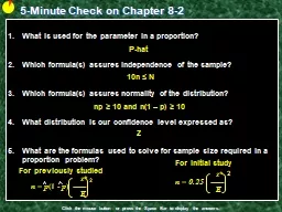
82 Click the mouse button or press the Space Bar to display the answers What is used for the parameter in a proportion Which formulas assures independence of the sample Which formulas assures normality of the distribution. Check. 1. . David baked 78 cookies for a bake sale. He set aside 12 cookies to share with volunteers. The remaining cookies are bagged with 3 cookies in each bag. How many bags does he have? . 2. A 3 lb. pork loin can be cut into 10 pork chops of equal weight. How many ounces are in each pork chop?. Find. Complete in your notes. . 1. . + . 2. - . . +(- . ). 3. - . . - . 4. - . . + (- . ). .  . 5 Minute Check. Find. Complete in your notes. . 1. . + . .  . 5 Minute Check. Find. Complete in your notes. . By. Laura A. Riffel, Ph.D.. Behavior Doctor Seminars. You will choose three or less behaviors to track . Type over the current letter with a new letter to stand for the behavior you are going to mark. Then type the word over the current word. The program will make the appropriate changes on the back side.. I pick an interesting passage or article to . read to the students. After I read . the . selection, students open their notebooks to the “Reading Minute” section. On a sheet of . notebook . paper, I have them write the day’s date and a one-sentence summary or thesis statement to remember . Tell whether each number is divisible by 2,3,4,5,6,9,10. You can use your rules sheet. . 1. 48. 2. 49. 3. 50. 4. 650. 5. 665. 6. 7,000. 5 Minute Check. Complete on the back of your homework.. Tell whether each number is divisible by 2,3,4,5,6,9,10.. notebook. Write an algebraic expression to represent the . following.. 1. Malinda goes bowling on Saturday. . . She bowls three games and pays $2 for . shoe . rental. . 2. Kyle has 5 more . than . one fourth as many . 1. s - . = . 2. s . = . 3. d 4 = 36. 4. d – 4 = 36.  . 5 Minute Check. Solve and show work on the back on your homework.. 1. s - . = .  . 5 Minute Check. Solve and show work on the back on your homework.. . 1. . . 2 4(7 – 3). 2. . -5 · (-4) 7. 3. . 4 – 1(-4). 4. . . 5 - 5³ (4 – 2). . 5 Minute Check. Find. Complete in your notes. . . 1. . . 2 4(7 – 3). . By. Laura A. Riffel, Ph.D.. Behavior Doctor Seminars. You will choose three or less behaviors to track . Type over the current letter with a new letter to stand for the behavior you are going to mark. Then type the word over the current word. The program will make the appropriate changes on the back side.. The One Minute Preceptor: Maintaining Efficiency While Teaching Jennifer Hagen, MD, FACP Office of Faculty Development University of Nevada, Reno School of Medicine Learning Objectives A pply the steps of the One Minute Preceptor Discover the truth and the facts about 15 Minute Manifestation™ PDF, eBook by Eddie Sergey. Click \"SHARE\" and \"DOWNLOAD\" to read the document offline. Conserve resources. with home energy . management. Managing home heat. Did . you know that the typical . U.S. family . spends about . $. 1,900 . a . year on home utility bills. ?. Source: US Department of Energy. 0 2 4 6 8 10 12 14 16 18 20 22 24 26 28 30 32 34 36 38 0 1 2 3 4 5 6 7 8 9 10 0 200 400 600 800 1000 1200 1400 1600 1800 Gallons Per Minute RPM D10 Performance 100 PSI (6.9 bar) 500 PSI (34.5 bar) 100 DOWNLOAD One Minute Herpes Cure PDF EBook ➤ Allison Freeman™ The Secret To Healing Virtually Every Type Of Herpes