/
Computing  Persistent  Homology Computing  Persistent  Homology

Computing Persistent Homology - PowerPoint Presentation

lindy-dunigan
lindy-dunigan . @lindy-dunigan
Follow
370 views
Uploaded On 2018-03-11

Computing Persistent Homology - PPT Presentation

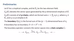
Matthew L Wright Institute for Mathematics and its Applications University of Minnesota Preliminaries Let be a simplicial complex and let be the twoelement field denotes the vector space generated by the ID: 647178

column simplex matrix simplices simplex column simplices matrix paired columns boundary homology positive reduced step negative number tree reduce total bit cycles

Share:

Link:

Embed:

Download Presentation from below link

Download Presentation The PPT/PDF document "Computing Persistent Homology" is the property of its rightful owner. Permission is granted to download and print the materials on this web site for personal, non-commercial use only, and to display it on your personal computer provided you do not modify the materials and that you retain all copyright notices contained in the materials. By downloading content from our website, you accept the terms of this agreement.


Presentation Transcript

Slide1

Computing

Persistent

Homology

Matthew L. Wright

Institute for Mathematics and its Applications

University of MinnesotaSlide2

Preliminaries

Let

be a simplicial complex, and let

be the two-element field.

denotes the vector space generated by the

-dimensional simplices of

.

consists of all -chains

, which are formal sums

, where

and

is a

-simplex in

.

The boundary

is the formal sum of the

-dimensional faces of

.

A boundary has no boundary:

.

The boundary operator connects the vector spaces into a chain complex :     


 Slide3

Preliminaries

The

-chains that have no boundary are called -cycles, and they form a subspace

of

.The

-chains that are the boundary of -chains are called

-boundaries, and they form a subspace

of .Since a boundary has no boundary,

.

The quotient

is the

th

homology group of

.The dimension of

is the th Betti

number of and is denoted

.

 Slide4

Computing

Betti

Numbers

Number the

-

simplices

of K consecutively from 1 to

.

The boundary matrix

records the face relationship for

-simplices and

-simplices.


if the

th

-simplex is a face of the th

-simplex

otherwise


Observe:  Thus,

.  

  Reduce to Smith normal form to obtain the desired ranks. 


 Slide5

Computing Persistent Homology

We start with a filtered

simplicial complex:


Step 1:

Sort the simplices to get a total ordering compatible with the

filtration.

Step 2: Obtain a boundary matrix

with respect to the total order on simplices.Step 3: Reduce the matrix using column additions, always respecting the total order on

simplices.Step 4: Read the persistence pairs to get the barcode.

 Slide6


Example:Slide7


Step 1:

Sort the simplices to get a total ordering compatible with the filtration

Compatible

means:

Simplices in each

precede simplices in

The faces of each simplex precede the simplex itself


Example:


 Slide8


Step 2:

Obtain a boundary matrix

with respect to the total order


Example:


if simplex is a codimension- face of simplex otherwise 


   Slide9


Example:


    Define to be the row number of the lowest non-zero entry in column . If column is empty, then

.  


 Example: and  Step 2: Obtain a boundary matrix with respect to the total order Slide10


Step 3:

Reduce the matrix

Example:


  for j = 1 to n: while ∃ j' < j with low(j') = low(j) ≠ 0: add column j' to column j


  ALGORITHM 

   Slide11


Step 4:

Read the persistence pairs

Example:


If , then simplex is negative, paired with simplex .If , then simplex is positive; look to row for pairing.If there is no with , then simplex generates homology in .

 Slide12


Example:


simplex : positive, unpairedsimplex : positive, paired with simplex simplex : positive, paired with simplex simplex : negative, paired with simplex simplex : negative, paired with simplex simplex : positive, paired with simplex simplex : negative, paired with simplex  Slide13


Example:


    simplex : positive, unpairedsimplex : positive, paired with simplex simplex : positive, paired with simplex simplex

: negative, paired with simplex simplex : negative, paired with simplex simplex : positive, paired with simplex simplex : negative, paired with simplex  bar in homology  simplices 2 and 4 enter at the same time, so the pair does not produce a barbar in homology bar

in homology Slide14


Example:


    bar in homology  

simplices 2 and 4 enter at the same time, so the pair does not produce a barbar in homology bar in homology  


  Now we can draw the barcode:Slide15

Data Structures

We store the matrix in a

column-sparse format

.

Store the matrix as an array of columns, and each column as a linked list.

The linked list for column

stores the row indexes of the nonzero entries in column

, in reverse order so that the “lowest” index is accessible at the beginning of the list.


1

2

3

4

5

6

7

2

1

3

1

3

265

4Slide16

Data Structures

Suppose we have reduced columns

through

. If

, we want to find

such that

.

To avoid looking through all columns

through , we use a low array

to store the index of each nonempty reduced column by low number. 

1

2

3

4

5

6

7

2

1

3

1

3

265412345

67low array45Slide17

Data Structures

Suppose we have reduced columns

through

. If

, we want to find

such that

.

To avoid looking through all columns

through , we use a low array

to store the index of each nonempty reduced column by low number. 

1

2

3

4

5

6

7

2

1

3

1

2

165412345

67low array45Slide18

Data Structures

Suppose we have reduced columns

through

. If

, we want to find

such that

.

To avoid looking through all columns

through

, we use a

low array to store the index of each nonempty reduced column by low number.


1

2

3

4

5

6

7

2

1

3

16541234567low array457Slide19

“Twist” Optimization

Observations:

If column

is reduced and

, then simplex

is negative, paired with positive simplex

.Then reducing column

will result in a column of zeros.If is the dimension of simplex

, then the dimension of simplex is

.


    Optimization: Reduce columns corresponding to higher-dimensional simplices first.If column is reduced and

, then set column to zero. reduced matrixSlide20

“Twist” Optimization

Example:

same boundary matrix as before


   First reduce columns corresponding to 2-simplices.Column is reduced, and .Thus, negative simplex is paired with positive simplex , so column must be zero.After reducing all columns corresponding to 2-simplices, then reduce columns corresponding to 1-simplices.Now we are done.

 unreduced matrixSlide21

Runtime Complexity

Let

be the total number of simplices, so is an

matrix.We must reduce

columns.Reducing any particular column requires at most

column additions.Each column addition requires at most operations.Therefore, the runtime is

.


number of column additions is


However, in practice, the runtime is often better than cubic.

Note that this complexity is just for the matrix reduction, and doesn’t include building the filtration or boundary matrix.Slide22

Generating Cycles

To find the cycles that represent homology classes, we must keep track of the column additions.

Consider the operation of adding column

to column :This is the same as adding the chain represented by column

to that represented by column .


This corresponds to multiplying on the right by the elementary matrix that has

s on the diagonal and in entry

.


 Slide23

Generating Cycles

Reducing

via column operations is the same as multiplying

on the right by matrix

.

Matrix is a product of elementary matrices and is upper triangular with

s on the diagonal.


 Slide24

Generating Cycles

The columns of

indicate the cycles and chains that kill cycles.

If column

in

is empty, then column in

gives the corresponding cycle.Otherwise, column in

gives the chain that kills the cycle corresponding to


 Slide25

Bit Tree

Replacing the linked lists (for columns) by a more clever data structure can make the algorithm faster, though the complexity is still

.

Bauer et. al. propose a bit tree: a 64-ary

tree, stored as an array. 

1

2

3

64

Each block has 64 bits. Bit

indicates whether the

th

subtree is non-empty.The leaves of the tree encode the nonzero entries of a column. Slide26

Bit Tree

1

2

3

64

The bit tree supports nearly constant time insertion, deletion, and lookup.

The “active” column is converted to a bit tree, then columns are added to it, and then it is converted back to a sparse structure.

Bauer et. al. recorded significant speed improvements when using the bit tree for column additions.Slide27

Available Software

JavaPlex

: http://git.appliedtopology.org/javaplex/Dionysus: http://www.mrzv.org/software/dionysus/

Perseus: http://www.sas.upenn.edu/~vnanda/perseus/Persistent Homology Algorithms Toolbox (PHAT): https://code.google.com/p/phat/Slide28

References

Ulrich Bauer, et. al. “PHAT – Persistent Homology Algorithms Toolbox.” http

://phat.googlecode.comHerbert Edelsbrunner and John Harer. “Persistent homology: a survey.” in

Surveys on discrete and computational geometry: twenty years later. AMS (2008).Afra Zomorodian and Gunnar Carlsson

. “Computing persistent homology.” Discrete and Computational Geometry. Vol. 33, no. 2 (2005), p. 249 – 274.