/
Lecture materials by Austin Troy Lecture materials by Austin Troy

Lecture materials by Austin Troy - PowerPoint Presentation

lindy-dunigan
lindy-dunigan . @lindy-dunigan
Follow
421 views
Uploaded On 2016-04-29

Lecture materials by Austin Troy - PPT Presentation

and Brian Voigt 2011 except where noted Lecture 6 Introduction to Projections and Coordinate Systems By Austin Troy and Brian Voigt University of Vermont with sections adapted from ESRIs online course on projections ID: 298723

austin lecture materials troy lecture austin troy materials brian voigt noted 2011 projection map surface area projections spheroid earth

Share:

Link:

Embed:

Download Presentation from below link

Download Presentation The PPT/PDF document "Lecture materials by Austin Troy" is the property of its rightful owner. Permission is granted to download and print the materials on this web site for personal, non-commercial use only, and to display it on your personal computer provided you do not modify the materials and that you retain all copyright notices contained in the materials. By downloading content from our website, you accept the terms of this agreement.


Presentation Transcript

Slide1

Lecture materials by Austin Troy and Brian Voigt © 2011, except where noted

Lecture 6:Introduction to Projections and Coordinate SystemsBy Austin Troy and Brian Voigt, University of Vermont,with sections adapted from ESRI’s online course on projections

------Using GIS--Slide2

The Earth’s Size and Shape

It is only relatively recently that we’ve been able to say what both areEstimates of shape by the ancients have ranged from a flat disk, to a cube to a cylinder to an oyster.Pythagoras was the first to postulate the Earth was a sphereBy the fifth century BCE, this was firmly established.But how big was it?

Lecture materials by Austin Troy

and Brian Voigt © 2011,

except where notedSlide3

The Earth’s Size

It was Posidonius who used the stars to determine the earth's circumference. “He observed that a given star could be seen just on the horizon at Rhodes. He then measured the star's elevation at Alexandria, Egypt, and calculated the angle of difference to be 7.5 degrees or 1/48th of a circle. Multiplying 48 by what he believed to be the correct distance from Rhodes to Alexandria (805 kilometers or 500 miles), Posidonius calculated the earth's circumference to be 38,647 kilometers (24,000 miles)--an error of only three percent.” -source: ESRI

Lecture materials by Austin Troy

and Brian Voigt © 2011,

except where notedSlide4

The Earth’s Shape

Earth is not a sphere, but an ellipsoid, because the centrifugal force of the earth’s rotation “flattens it out”.

This was finally proven by the French in 1753

The earth rotates about its shortest axis, or minor axis, and is therefore described as an

oblate ellipsoid

Source: ESRI

Lecture materials by Austin Troy

and Brian Voigt © 2011,

except where notedSlide5

The Earth’s Shape

Because it’s so close to a sphere, the Earth is often referred to as a spheroid: that is a type of ellipsoid that is really, really close to being a sphere

These are two common spheroids used today:

the difference between its major axis and its minor axis is less than 0.34%.

Source: ESRI

Lecture materials by Austin Troy

and Brian Voigt © 2011,

except where notedSlide6

SpheroidsThe International 1924 and the Bessel 1841 spheroids are used in Europe while in North America the GRS80, and decreasingly, the Clarke 1866 Spheroid, are usedIn Russia and China the Krasovsky spheroid is used and in India the Everest spheroid

Lecture materials by Austin Troy and Brian Voigt © 2011, except where notedSlide7

SpheroidsTwo common spheroids use slightly different major and minor axis lengths

Source: ESRI

Lecture materials by Austin Troy

and Brian Voigt © 2011,

except where notedSlide8

SpheroidsOne more thing about spheroids: If your mapping scales are smaller than 1:5,000,000 (small scale maps), you can use an authalic sphere to define the earth's shape to make things more simpleFor maps at larger scale (most of the maps we work with in GIS), you generally need to employ a spheroid to ensure accuracy and avoid positional errors

Lecture materials by Austin Troy and Brian Voigt © 2011, except where notedSlide9

GeoidWhile the spheroid represents an idealized model of the earth’s shape, the geoid represents the “true,” highly complex shape of the earth, which, although “spheroid-like,” is actually very irregular at a fine scale of detail, and can’t be modeled with a formula (the DOD tried and gave up after building a model of 32,000 coefficients)It is the 3 dimensional surface of the earth along which the pull of gravity is a given constant; ie. a standard mass weighs an identical amount at all points on its surface The gravitational pull varies from place to place because of differences in density, which causes the geoid to bulge or dip above or below the ellipsoidOverall these differences are small ~ 100 meters

Lecture materials by Austin Troy and Brian Voigt © 2011, except where notedSlide10

Geoid

www.esri.com/news/arcuser/0703/geoid1of3.html

The geoid is actually measured and interpolated, using gravitational measurements.

Lecture materials by Austin Troy

and Brian Voigt © 2011,

except where notedSlide11

Spheroids and GeoidsWe have several different estimates of spheroids because of irregularities in the earth surface: there are slight deviations and irregularities in different regionsBefore remote satellite observation, had to use a different spheroid for different regions to account for irregularities (see Geoid, ahead) to avoid positional errorsThat is, continental surveys were isolated from each other, so ellipsoidal parameters were fit on each continent to create a spheroid that minimized error in that region, and many stuck with those for years

Lecture materials by Austin Troy and Brian Voigt © 2011, except where notedSlide12

The Geographic GridOnce you have a spheroid, you also define the location of poles (axis points of revolution) and equator (midway circle between poles, spanning the widest dimension of the spheroid), you have enough information to create a coordinate grid or “graticule” for referencing the position of features on the spheroid.

Lecture materials by Austin Troy and Brian Voigt © 2011, except where notedSlide13

The Geographic GridThis is a location reference system for the earth’s surface, consisting of:Meridians: lines of longitude andParallels: lines of latitude

Source: ESRI

Prime meridian is at

0º longitude (Greenwich, England)

Equator is at 0º latitude

Lecture materials by Austin Troy

and Brian Voigt © 2011,

except where notedSlide14

The Geographic GridThis is like a planar coordinate system, with an origin at the point where the equator meets the prime meridianThe difference is that it is not a grid because grid lines must meet at right angles; this is why it’s called a graticule insteadEach degree of latitude represents about 110 km, although, that varies slightly because the earth is not a perfect sphere

Lecture materials by Austin Troy and Brian Voigt © 2011, except where notedSlide15

The Geographic GridLatitude and longitude can be measured either in degrees, minutes, seconds (e.g. 56° 34’ 30”), where minutes and seconds are base-60 (like on a clock)Can also use decimal degrees (more common in GIS), where minutes and seconds are converted to a decimalExample: 45° 52’ 30” = 45.875 °

Lecture materials by Austin Troy

and Brian Voigt © 2011,

except where notedSlide16

The Geographic GridLatitude lines form parallel circles of different sizes, while longitude lines are half-circles that meet at the polesLatitude goes from 0 to 90º N or S and longitude to 180 º E or W of meridian; the 180 º line is the date line

Source: ESRI

Lecture materials by Austin Troy

and Brian Voigt © 2011,

except where notedSlide17

DatumsThree dimensional surface from which latitude, longitude and elevation are calculatedAllows us to figure out where things actually are on the graticule since the graticule only gives us a framework for measuring, not actual locationsFrame of reference for placing specific locations at specific points on the spheroidDefines the origin and orientation of latitude and longitude lines.

Lecture materials by Austin Troy and Brian Voigt © 2011, except where notedSlide18

Datums A datum is essentially the model that is used to translate a spheroid into locations on the earthA spheroid only gives you a shape—a datum gives you locations of specific places on that shape. Hence, a different datum is generally used for each spheroidTwo things are needed for datum: spheroid and set of surveyed and measured points

Lecture materials by Austin Troy and Brian Voigt © 2011, except where notedSlide19

Surface-Based DatumsPrior to satellites, datums were realized by connected series of ground-measured survey monuments A central location was chosen where the spheroid meets the earth: this point was intensively measured using pendulums, magnetometers, sextants, etc. to try to determine its precise location. Originally, the “datum” referred to that “ultimate reference point.” Eventually the whole system of linked reference and sub-refence points came to be known as the datum.

Lecture materials by Austin Troy

and Brian Voigt © 2011,

except where notedSlide20

Surface-Based DatumsStarting points need to be very central relative to landmass being measuredIn NAD27 center point was Mead’s Ranch, KS NAD27 resulted in lat/long coordinates for about 26,000 survey points in the US and Canada.Limitation: requires line of sight, so many survey points requiredProblem: errors compound with distance

Lecture materials by Austin Troy and Brian Voigt © 2011,

except where notedSlide21

c

Surface-Based DatumsThese were largely done without having to measure distances. How?Using high-quality celestial observations and distance measurements for the first two observations, could then use trigonometry to determine distances.

a

b

A

With b and c and A known,

determine

a’s location through solving for B and C by the law of

sines

B=A(sin(b))/(sin(a))

B

C

D

E

Mead’s Ranch

Secondary

Measured

point

Lecture materials by Austin Troy

and Brian Voigt © 2011,

except where notedSlide22

Satellite-Based DatumsCenter of the spheroid can be matched with the center of the earth.Satellites started collecting geodetic information in 1962 as part of National Geodetic SurveyYields a spheroid that when used as a datum correctly maps the earth such that all lat / lon measurements from all maps created with that datum agree.Rather than linking points through surface measures to initial surface point, are measurements are linked to reference point in outer space

Lecture materials by Austin Troy

and Brian Voigt © 2011,

except where notedSlide23

Common DatumsPreviously, the most common spheroid was Clarke 1866; the North American Datum of 1927 (NAD27) is based on that spheroid, and has its center in Kansas.NAD83 is the new North American datum (for Canada / Mexico too) based on the GRS80 geocentric spheroid. It is the official datum of the USA, Canada and Central AmericaWorld Geodetic System 1984 (WGS84) is newer spheroid / datum, created by the US DOD; it is more or less identical to Geodetic Reference System 1980 (GRS80). GPS uses WGS84

Lecture materials by Austin Troy

and Brian Voigt © 2011,

except where notedSlide24

Lat / Long and DatumsPre-satellite datums are surface-based. A given datum has the spheroid meet the earth in a specified location.Datum is most accurate near the contact point, less accurate as move away (remember, this is different from a projection surface because the ellipsoid is 3D).

Lecture materials by Austin Troy and Brian Voigt © 2011, except where notedSlide25

Lat / Long and DatumsLat / long coordinates calculated with one datum are valid only with reference to that datum.This means those coordinates calculated with NAD27 are in reference to a NAD27 earth surface, not a NAD83 earth surface.Example: the DMS control point in Redlands, CA is -117º 12’ 57.75961”, 34 º 01’ 43.77884” in NAD83 and -117º 12’ 54.61539” 34 º 01’ 43.72995” in NAD27Click here for a chart of the different coordinates for the Capital Dome center under different datums (Peter Dana)

Lecture materials by Austin Troy and Brian Voigt © 2011, except where notedSlide26

Datum ShiftWhen we go from a surface-oriented datum to a spheroid-based datum, the estimated position of survey benchmarks improves; this is called datum shiftThat shift varies with location: 10 to 100 m in the continental US, 400 m in Hawaii, 35 m in Vermont

Source: http

://www.ngs.noaa.gov/TOOLS/Nadcon/Nadcon.html

Lecture materials by Austin Troy

and Brian Voigt © 2011,

except where notedSlide27

Map ProjectionThis is the method by which we transform the earth’s spheroid (real world) to a flat surface (abstraction), either on paper or digitallyBecause we can’t take our globe everywhere with us!Remember: most GIS layers are 2-D

3D

2D

Think about projecting a

globe

onto a wall

Source: ESRI

Lecture materials by Austin Troy

and Brian Voigt © 2011,

except where notedSlide28

Map Projection

The earliest and simplest map projection is the plane chart, or plate carrée, invented around the first century; it treated the graticule as a grid of equal squares, forcing meridians and parallels to meet at right angles

If applied to the world as mapped now, it would look like

:

Lecture materials by Austin Troy

and Brian Voigt © 2011,

except where notedSlide29

Map Projection: DistortionBy definition, projections distorts:Shape Area Distance DirectionSome projections specialize in preserving one or several of these features, but none preserve all

Lecture materials by Austin Troy and Brian Voigt © 2011, except where notedSlide30

Shape DistortionShape: projection can distort the shape of a feature. Conformal maps preserve the shape of smaller, local geographic features, while general shapes of larger features are distorted. That is, they preserve local angles; angle on map will be same as angle on globe. Conformal maps also preserve constant scale locally.

Lecture materials by Austin Troy and Brian Voigt © 2011, except where notedSlide31

Shape Distortion

Mercator (left)

World Cylindrical Equal Area (above)

The distortion in shape above is necessary to get Greenland to have the correct area;

The Mercator map looks good but Greenland is many times too big

Lecture materials by Austin Troy

and Brian Voigt © 2011,

except where notedSlide32

Area DistortionArea: projection can distort the property of equal area (or equivalent), meaning that features have the correct area relative to one another.Map projections that maintain this property are often called equal area map projections.For instance, if S America is 8x larger than Greenland on the globe, it will be 8x larger on mapNo map projection can have conformality and equal area >>> sacrifice shape to preserve area and vice versa.

Lecture materials by Austin Troy

and Brian Voigt © 2011,

except where notedSlide33

Area Distortion827,000 square miles6.8 million square miles

Mercator Projection

Lecture materials by Austin Troy

and Brian Voigt © 2011,

except where notedSlide34

Distance DistortionDistance: projection can distort measures of true distance. Accurate distance is maintained for only certain parallels or meridians unless the map is localized. Maps are said to be equidistant if distance from the map projection's center to all points is accurate.

Lecture materials by Austin Troy and Brian Voigt © 2011, except where notedSlide35

Distance Distortion

4,300 km: Robinson

5,400 km: Mercator

Lecture materials by Austin Troy

and Brian Voigt © 2011,

except where notedSlide36

Direction DistortionDirection: projection can distort true directions between geographic locations; that is, it can mess up the angle, or azimuth between two features. Some azimuthal map projections maintain the correct azimuth between any two points. In a map of this kind, the angle of a line drawn between any two locations on the projection gives the correct direction with respect to true north.

Lecture materials by Austin Troy and Brian Voigt © 2011, except where notedSlide37

Map Projection: DistortionWhen choosing a projection, one must take into account what it is that matters in your analysis and what properties you need to preserve.Conformal and equal area properties are mutually exclusive but some map projections can have more than one preserved property. For instance a map can be conformal and azimuthal.Conformal and equal area properties are global (apply to whole map) while equidistant and azimuthal properties are local and may be true only from or to the center of map.

Lecture materials by Austin Troy and Brian Voigt © 2011, except where notedSlide38

Projection Specific DistortionMercator maintains shape and direction, but sacrifices area accuracy.The Sinusoidal and Equal-Area Cylindrical projections both maintain area, but look quite different from each other. The latter distorts shape.The Robinson projection does not enforce any specific properties but is widely used because it makes the earth’s surface and its features look somewhat accurate.

Lecture materials by Austin Troy and Brian Voigt © 2011, except where notedSlide39

Projection Specific Distortion

Lecture materials by Austin Troy and Brian Voigt © 2011, except where noted

Mercator—goes on forever

Robinson

SinusoidalSlide40

Quantifying DistortionTissot’s indicatrix, made up of ellipses, is a method for measuring distortion of a map; here is Robinson

Lecture materials by Austin Troy and Brian Voigt © 2011, except where notedSlide41

Quantifying Distortion

Sinusoidal

Area of these ellipses should be same as those at equator, but shape is different

Lecture materials by Austin Troy

and Brian Voigt © 2011,

except where notedSlide42

Map Projection: Cylindrical

Created by wrapping a cylinder around a globeThe meridians (longitude) in cylindrical projections are equally spaced, while the spacing between parallel lines (latitude) increases toward the polesMeridians never converge so poles can’t be shown

Source: ESRI

Lecture materials by Austin Troy

and Brian Voigt © 2011,

except where notedSlide43

Cylindrical Map Types

Tangent to great circle: in the simplest case, the cylinder is North-South, so it is tangent (touching) at the equator; this is called the standard parallel and represents where the projection is most accurateIf the cylinder is smaller than the circumference of the earth, then it intersects as a secant in two places

Source: http://nationalatlas.gov/articles/mapping/a_projections.html

Lecture materials by Austin Troy

and Brian Voigt © 2011,

except where notedSlide44

Cylindrical Map TypesSecant projections are more accurate because projection is more accurate the closer the projection surface is to the globe and a when the projection surface touches twice, that means it is on average closer to the globeThe distance from map surface to projection surface is described by a scale factor, which is 1 where they touch

Earth surface

Projection surface

0.9996

Central meridian

Standard meridians

Lecture materials by Austin Troy

and Brian Voigt © 2011,

except where notedSlide45

Cylindrical Map Types3. Transverse cyclindrical projections: in this type the cylinder is turned on its side so it touches a line of longitude; these can also be tangent

Lecture materials by Austin Troy and Brian Voigt © 2011, except where notedSlide46

Cylindrical Map Distortion

A north-south cylindrical Projections cause major distortions in higher latitudes because those points on the cylinder are further away from from the corresponding point on the globeScale is constant in north-south direction and in east west direction along the equator for an equatorial projection but non constant in east-west direction as move up in latitudeRequires alternating Scale Bar based on latitude

Lecture materials by Austin Troy

and Brian Voigt © 2011,

except where notedSlide47

Cylindrical Map Distortion

If such a map has a scale bar, know that it is only good for those places and directions in which scale is constant—the equator and the meridiansHence, the measured distance between Nairobi and the mouth of the Amazon might be correct, but the measured distance between Toronto and Vancouver would be off; the measured distance between Alaska and Iceland would be even further off

Lecture materials by Austin Troy

and Brian Voigt © 2011,

except where notedSlide48

Cylindrical Map Distortion

X miles

0

atitude

25

latitude

50

latitude

Lecture materials by Austin Troy

and Brian Voigt © 2011,

except where notedSlide49

Cylindrical Map Distortion

Why is this? Because meridians are all the same length, but parallels are not.This sort of projection forces parallels to be same length so it distorts them As move to higher latitudes, east-west scale increases (2 x equatorial scale at 60° N or S latitude) until reaches infinity at the poles; N-S scale is constantSlide50

Map Projection: Conic

Projects a globe onto a coneIn simplest case, globe touches cone along a single latitude line, or tangent, called standard parallelOther latitude lines are projected onto coneTo flatten the cone, it must be cut along a line of longitude (see image)

The opposite line of longitude is called the

central

meridian

Source: ESRI

Lecture materials by Austin Troy

and Brian Voigt © 2011,

except where notedSlide51

Map Projection: Conic

Is most accurate where globe and cone meet—at the standard parallelDistortion generally increases north or south of it, so poles are often not includedConic projections are typically used for mid-latitude zones with east-to-west orientation. They are normally applied only to portions of a hemisphere (e.g. North America)

Lecture materials by Austin Troy

and Brian Voigt © 2011,

except where notedSlide52

Map Projection: Conic

Can be tangent or secantSecants are more accurate for reasons given earlier

Lecture materials by Austin Troy

and Brian Voigt © 2011,

except where notedSlide53

Map Projection: Planar /AzimuthalProject a globe onto a flat planeThe simplest form is only tangent at one pointAny point of contact may be used but the poles are most commonly used

Source: ESRI

Lecture materials by Austin Troy

and Brian Voigt © 2011,

except where notedSlide54

When another location is used, it is generally to make a small map of a specific areaWhen the poles are used, longitude lines look like hub and spokesBecause the area of distortion is circular around the point of contact, they are best for mapping roughly circular regions, and hence the poles

Source: ESRI

Map Projection: Planar /Azimuthal

Lecture materials by Austin Troy

and Brian Voigt © 2011,

except where notedSlide55

Map Projection: Mercator

Specific type of cylindrical projectionInvented by Gerardus Mercator during the 16th CenturyIt was invented for navigation because it preserves azimuthal accuracy—that is, if you draw a straight line between two points on a map created with Mercator projection, the angle of that line represents the actual bearing you need to sail to travel between the two points

Source: ESRI

Lecture materials by Austin Troy

and Brian Voigt © 2011,

except where notedSlide56

Map Projection: MercatorNot so good for preserving areaEnlarges high latitude features like Greenland & Antarctica and shrinks mid latitude features.

Lecture materials by Austin Troy

and Brian Voigt © 2011,

except where notedSlide57

Map Projection:Transverse Mercator

Invented by Johann Lambert in 1772, this projection is cylindrical, but the axis of the cylinder is rotated 90°, so the tangent line is longitudinal, rather than the equator In this case, only the central longitudinal meridian and the equator are straight lines

All other lines are represented by complex curves: that is they can’t be represented by single section of a circle

Source: ESRI

Lecture materials by Austin Troy

and Brian Voigt © 2011,

except where notedSlide58

Map Projection:Transverse MercatorTransverse Mercator projection is not used on a global scale but is applied to regions that have a general north-south orientation, while Mercator tends to be used more for geographic features with east-west axis.Commonly used in the US with the State Plane Coordinate system, with north-south features

Lecture materials by Austin Troy and Brian Voigt © 2011, except where notedSlide59

Lecture materials by Austin Troy © 2008, except where noted

Map Projection:Lambert Conformal Conic

Invented

in 1772, this is a form of a conic projection

Latitude lines are unequally spaced arcs that are portions of concentric circles. Longitude lines are actually radii of the same circles that define the latitude lines.

Source: ESRISlide60

Map Projection:Lambert Conformal ConicVery good for middle latitudes with east-west orientation. It portrays the pole as a pointIt portrays shape more accurately than area and is commonly used for North America. The State Plane coordinate system uses it for east-west oriented features

Lecture materials by Austin Troy and Brian Voigt © 2011, except where notedSlide61

Map Projection:Lambert Conformal Conic

A slightly more complex form of conic projection because it intersects the globe along two lines, called secants, rather than along one, which would be called a tangentThere is no distortion along those two linesDistortion increases with distance from secants

Source: ESRI

Lecture materials by Austin Troy

and Brian Voigt © 2011,

except where notedSlide62

Map Projection: Albers Equal Area Conic

Developed by Heinrich Christian Albers in the early nineteenth century for European mapsConic projection, using secants as standard parallelsDifferences between Albers and Lambert Lambert preserves shape Albers preserves areaPoles are not represented as points, but as arcs, meaning that meridians don’t convergeLatitude lines are unequally spaced concentric circles, whose spacing decreases toward the poles. Useful for portraying large land units, like Alaska or all 48 states

Lecture materials by Austin Troy

and Brian Voigt © 2011,

except where notedSlide63

Map Projection: Albers Equal Area Conic

Preserves area by making the scale factor of a meridian at any given point the reciprocal of that along the parallel. Scale factor is the ratio of local scale of a point on the projection to the reference scale of the globe; 1 means the two are touching and greater than 1 means the projection surface is at a distance

Lecture materials by Austin Troy

and Brian Voigt © 2011,

except where notedSlide64

Other Selected Projections

More Cylindrical equal area: (have straight meridians and parallels, the meridians are equally spaced, the parallels unequally spaced) Behrmann cyclindrical equal-area: single standard parallel at 30 ° northGall’s stereographic: secant intersecting at 45° north and 45 ° southPeter’s:

de-emphasizes area exaggerations in high latitudes; standard parallels at 45 or 47

°

Thanks to Peter Dana,

The Geographer's Craft Project, Department of Geography, The University of Colorado at Boulder

for links

Lecture materials by Austin Troy

and Brian Voigt © 2011,

except where notedSlide65

Other Selected Projections

Azimuthal projections:Azimuthal equidistant: preserves distance property; used to show air route distancesLambert Azimuthal equal area: Often used for polar regions; central meridian is straight, others are curvedOblique Aspect OrthographicNorth Polar Stereographic

Thanks to Peter Dana,

The Geographer's Craft Project, Department of Geography, The University of Colorado at Boulder

for links

Lecture materials by Austin Troy

and Brian Voigt © 2011,

except where notedSlide66

Other Selected Projections

More conic projectionsEquidistant Conic: used for showing areas near to, but on one side of the equator, preserves only distance propertyPolyconic: used for most of the early USGS quads; based on an infinite number of cones tangent to an infinite number of parallels; central meridian straight but other lines are complex curves

Thanks to Peter Dana,

The Geographer's Craft Project, Department of Geography, The University of Colorado at Boulder

for links

Lecture materials by Austin Troy

and Brian Voigt © 2011,

except where notedSlide67

Other Selected Projections

Pseudo-cylindrical projections: resemble cylindrical projections, with straight, parallel parallels and equally spaced meridians, but all meridians but the reference meridian are curvesMollweide: used for world maps; is equal-area; 90th meridians are semi-circles Robinson:based on tables of coordinates, not mathematical formulas; distorts shape, area, scale, and distance in an attempt to make a balanced map

Thanks to Peter Dana,

The Geographer's Craft Project, Department of Geography, The University of Colorado at Boulder

for links

Lecture materials by Austin Troy

and Brian Voigt © 2011,

except where notedSlide68

Coordinate Systems

Map projections provide the means for viewing small-scale maps, such as maps of the world or a continent or country (1:1,000,000 or smaller)Plane coordinate systems are typically used for much larger-scale mapping (1:100,000 or bigger)

Lecture materials by Austin Troy

and Brian Voigt © 2011,

except where notedSlide69

Coordinate Systems

Projections are designed to minimize distortions of the four properties we talked about, because as scale decreases, error increasesCoordinate systems are more about accurate positioning (relative and absolute positioning) To maintain their accuracy, coordinate systems are generally divided into zones where each zone is based on a separate map projection

Lecture materials by Austin Troy

and Brian Voigt © 2011,

except where notedSlide70

Reason for PCSs

Remember from before that projections are most accurate where the projection surface is close to the earth surface. The further away it gets, the more distorted it gets

Hence a global or even continental projection is bad for accuracy because it’s only touching along one (tangent) or two (secant) lines and gets increasingly distorted

Lecture materials by Austin Troy

and Brian Voigt © 2011,

except where notedSlide71

Reason for PCSs

Plane coordinate systems get around this by breaking the earth up into zones where each zone has its own projection center and projection. The more zones there are and the smaller each zone, the more accurate the resulting projections This serves to minimize the scale factor, or distance between projection surface and earth surface to an acceptable level

Lecture materials by Austin Troy

and Brian Voigt © 2011,

except where notedSlide72

Coordinate Systems

The four most commonly used coordinate systems in the US:Universal Transverse Mercator (UTM) grid systemState Plane Coordinate System (SPC)Others:The Universal Polar Stereographic (UPS) grid systemThe Public Land Survey System (PLSS)

Lecture materials by Austin Troy

and Brian Voigt © 2011,

except where notedSlide73

UTM

Universal Transverse MercatorUTM is based on the Transverse Mercator projection (remember, that’s using a cylinder turned on its side)It generally uses either the NAD27 or NAD83 datums, so you will often see a layer as projected in “UTM83” or “UTM27”UTM is used for large scale mapping applications the world over, when the unit of analysis is fairly small, like a state

Lecture materials by Austin Troy

and Brian Voigt © 2011,

except where notedSlide74

UTM

UTM divides the earth between 84°N and 80°S into 60 zones, each of which covers 6 degrees of longitudeZone 1 begins at 180 ° W longitude.Each UTM zone is projected separately There is a false origin (zero point) in each zone

Lecture materials by Austin Troy

and Brian Voigt © 2011,

except where notedSlide75

United States UTM Zones

Lecture materials by Austin Troy and Brian Voigt © 2011, except where notedSlide76

UTM

Scale factors are 0.9996 in the middle and 1 at the secantsIn the Transverse Mercator projection, the “cylinder” touches at two secants, so there is a slight bulge in the middle, at the central meridian. This bulge is very very slight, so the scale factor is only 0.9996

Earth surface

Projection surface

0.9996

Central meridian

Standard meridians

Lecture materials by Austin Troy

and Brian Voigt © 2011,

except where notedSlide77

UTM

In the northern hemisphere, coordinates are measured from a false origin at the equator and 500,000 meters west of the central meridianIn the southern hemisphere, coordinates are measured from a false origin 10,000,000 meters south of the equator and 500,000 meters west of the central meridianAccuracy: 1 in 2,500

Lecture materials by Austin Troy

and Brian Voigt © 2011,

except where notedSlide78

UTM

Because each zone is big, UTM can result in significant errors as get further away from the center of a zone, corresponding to the central line

Lecture materials by Austin Troy

and Brian Voigt © 2011,

except where notedSlide79

SPC System

State Plane Coordinate System is one of the most common coordinate systems in use in the USIt was developed in the 1930s to record original land survey monument locations in the USMore accurate than UTM, with required accuracy of 1 part in 10,000Zones are much smaller—many states have two or more zones

Lecture materials by Austin Troy

and Brian Voigt © 2011,

except where notedSlide80

SPC System

Transverse Mercator projection is used for zones that have a north south access. Lambert conformal conic is used for zones that are elongated in the east-west direction. Why?Units of measurement are feet, which are measured from a false origin. SPC maps are found based on both NAD27 and NAD83, like with UTM, but SPC83 is in meters, while SPC27 is in feet

Lecture materials by Austin Troy

and Brian Voigt © 2011,

except where notedSlide81

SPC System

Many States have their own version of SPCVermont has the Vermont State Plane Coordinate System, which is in meters and based on NAD83In 1997, VCGI converted all their data from SPC27 to SPC83Vermont uses Transverse Mercator because of its north-south orientation

Lecture materials by Austin Troy

and Brian Voigt © 2011,

except where notedSlide82

State Plane Zone Map of New Englandhttp://www.ems-i.com/smshelp/General_Tools/Coordinates/new_england_state_plane.htm

Lecture materials by Austin Troy and Brian Voigt © 2011,

except where notedSlide83

State Plane Zone Map of the Northwesthttp://www.ems-i.com/smshelp/General_Tools/Coordinates/northwest_state_plane.htm

Lecture materials by Austin Troy and Brian Voigt © 2011,

except where notedSlide84

SPC System

Note how a conic projection is used here, since the errors indicate an east-west central line

Polygon errors-state plane

Lecture materials by Austin Troy

and Brian Voigt © 2011,

except where noted