PDF-Correcting the MSU Middle Tropospheric Temperature for Diurnal Drifts

Author : lois-ondreau | Published Date : 2016-03-18

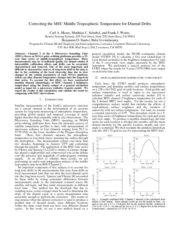
Fig 1 Example simulated MSU Channel 2 diurnal cycles calculated fromhourly CCM3 output These diurnal cycles are for the month of June aand c are for a 25 x 25degree

Presentation Embed Code

<iframe width="560" height="315" src="https://www.docslides.com/embed/260327" frameborder="0" allowfullscreen></iframe>

Download Presentation

Download Presentation The PPT/PDF document "Correcting the MSU Middle Tropospheric T..." is the property of its rightful owner. Permission is granted to download and print the materials on this website for personal, non-commercial use only, and to display it on your personal computer provided you do not modify the materials and that you retain all copyright notices contained in the materials. By downloading content from our website, you accept the terms of this agreement.

Correcting the MSU Middle Tropospheric Temperature for Diurnal Drifts: Transcript

Download Document

Here is the link to download the presentation.
"Correcting the MSU Middle Tropospheric Temperature for Diurnal Drifts"The content belongs to its owner. You may download and print it for personal use, without modification, and keep all copyright notices. By downloading, you agree to these terms.