In order for a diver to do what he or she does the diver applies effective torques at the joints We want to find a recipe for doing this that will cause the simulated diver to execute the diver ID: 582450
Download Presentation The PPT/PDF document "Lecture 26. Control of the Diver" is the property of its rightful owner. Permission is granted to download and print the materials on this web site for personal, non-commercial use only, and to display it on your personal computer provided you do not modify the materials and that you retain all copyright notices contained in the materials. By downloading content from our website, you accept the terms of this agreement.
Slide1
Lecture 26. Control of the Diver
In order for a diver to do what he or she does the diver applies effective torques at the joints
We want to find a recipe for doing this that will cause the simulated diver to execute the diver
This is a control problem
1Slide2
2
Tomorrow’s office hours will be1:30 to 3:30
I have to leave at 3:30Slide3
We have a special case of nonlinear control here and I want to explore that, beginning with some discussion
and then some simpler models3Slide4
4
Suppose we want the solution of a second order system to follow some prescription
We can write the second order system
The error
can be made to satisfy the homogeneous equation
by the proper choice of
f
(
t
)Slide5
5
choose
then
is the desired error equationSlide6
6
This can be extended to a quasilinear system, which is what we typically have
converts the nonlinear equation to the linear form that yields a decaying error
given
this choice for
f
(
t
)
This is called
feedback linearizationSlide7
7
What are we doing here?
We are asking that
become
and we choose the forcing function to make this happen
This is cool, but it’s only 1D — what happens in a coupled system?Slide8
8
For the class of problems we are considering, which includes divers and some robots, we can choose the generalized coordinates such that each external force appears in only one reduced Hamilton equation
This is not necessary, but it cleans up the algebra
and I’ll assume we’ve taken the trouble to do that, so my simplest coupled case isSlide9
9
substitute
into the system and solve for
f
1
and
f
2
When these are substituted back into the original equations we obtainSlide10
10
and if the system is not singular
then the identical parenthetical equations must equal zero:
the errors vanish asymptoticallySlide11
11
This looks like magic, but it isn’t
To make this work we have a necessary condition: as many forces as controlled variables
There’re more, but I can’t give them all to you.
It works for sufficiently simple systems with only revolute joints —
divers and many robots (not the Stanford arm)
I’d like to look at the inverted double pendulum from this perspective
before moving on to more complicated systemsSlide12
12
Planar inverted double pendulum: base fixed to the ground
parameters:
l1, l2
m
1
,
m
2
I treat them as slender
membersSlide13
13
We know how the double pendulum goes
Six holonomic constraints to restrict it to the
x = 0 plane
Four connectivity constraints relating
CMs
to the ground
Apply all ten constraints and define a two dimensional
qSlide14
14
We can form a LagrangianSlide15
15
There are no additional constraints, so we can let qdot equal u
We can find p
and then the pieces of Hamilton’s equationsSlide16
16Slide17
17
We have four differential equations and seven algebraic equations
(We can actually look at these in the Mathematica notebook)
The next issue is designing the control
so by assigning
we assign Slide18
18
We can look at various desired angles, both steady and time-dependent
Here’s the algorithm for vertical stabilizationSlide19
19
and the resultSlide20
20
Here we ask both links to follow sinusoidal paths out of phaseSlide21
21
and here’s the result of thatSlide22
22
Here are the torques required to perform the tracking shown on the previous slideSlide23
23
How about a simple diving problem — a three link diver?Slide24
24
Three links —> 18 variables
Confine to the x constant plane —> nine variables
Four connectivity constraints —> five variables
Number the links from the bottom to the top
and select the middle link as the reference linkSlide25
25
There are two torques — one at each joint — as shown in the sketch and we want to choose our variables accordinglySlide26
26
We get the Lagrangian as usualSlide27
27
This is a fancy torque, suitable for 3D
but of course only two of the components actually do anything
The important thing is that the choice of
q
has isolated the two torquesSlide28
28
Note that we have written this in terms of the desired
qs, not the yi
The next slide shows the development of the
Z
s and their gradientsSlide29
29Slide30
30
We need the symbolic versions to build the equations we intend to integrateSlide31
31Slide32
32
The two internal angles start at zero, go to a maximum of 2π/3, and back to zero in the time interval tf
Midway through the ends of the two outboard links should touch
We can do this integration and see what the results are
We can start by looking at the closest approach, when the two links are to touchSlide33
33Slide34
34Slide35
35Slide36
36Slide37
37Slide38
38
It is now probably worth looking at the Mathematica notebooks