PDF-WAVEFORM ANALYSIS TECHNIQUES IN AIRBORNE LASER SCANNING W. Wagner, A.

Author : lois-ondreau | Published Date : 2015-12-05

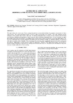
IAPRS Volume XXXVI Part 3 W52 2007 413 on smallfootprint waveform data can still be considered to be only in its beginning a number of benefits start to emerge

Presentation Embed Code

Download Presentation

Download Presentation The PPT/PDF document "WAVEFORM ANALYSIS TECHNIQUES IN AIRBORNE..." is the property of its rightful owner. Permission is granted to download and print the materials on this website for personal, non-commercial use only, and to display it on your personal computer provided you do not modify the materials and that you retain all copyright notices contained in the materials. By downloading content from our website, you accept the terms of this agreement.

WAVEFORM ANALYSIS TECHNIQUES IN AIRBORNE LASER SCANNING W. Wagner, A.: Transcript

IAPRS Volume XXXVI Part 3 W52 2007 413 on smallfootprint waveform data can still be considered to be only in its beginning a number of benefits start to emerge Jutzi and Stilla 2003 point out. tuwienacat cbipftuwienacat Christian Doppler Laboratory Spatial Data from Laser Scanning and Remote Sensing KEY WORDS Airborne Laser Scanning Terrestrial Laser Scanning LiDAR Geometry Orientation Registration Segmentation Calibration Digital Terrain the Marshall testbed. Ethan Gutmann, Bruce Baker, Roy Rasmussen, John . Kochendorfer. , . David . Gochis. , Scott . Landolt. , Tilden Meyers, Kristine Larson. 5/25/2011. Snow measurement importance. Which size snowplow would you want? . Cores and Drill Chips. to Complement Spectral Measures. Thomas BELLIGOÏ. Erick RAMANAIDOU. & Eric PIRARD. Liege. City. The . cradle. of . coal. . mining. , . steelmaking. and zinc . metallurgy. ServicesEngineering As-Built FacilitiesMeji Riser Platform Meji Production Platform Meji Gas Gathering Compression PlatformSafety RecordZero LTI Zero MTICompleted Q4 2018Nigeria West Africawwwarioshc BIM Engineering US is a leading Building Information Technology solution service provider offering end-to-end solutions in Mechanical, Electrical, Plumbing, and Fire Protection systems engineering, design, and construction. The availability of a wide range of companies providing 3D laser scanning services, selecting the right one can be tough. Here are some tips that can help you make a perfect choice. 3D mapping or scanning has become a crucial component in engineering, construction, and architecture. Here are a few significant benefits of 3D laser scanning that you should know. Aerial solutions and 3D laser scanning technologies have revolutionized the world of industrial inspections, construction projects, restoration, and more. Wondering how these technologies unleash new possibilities for achieving once-deemed impossible things? Read here. Have you ever wondered how laser scanning can benefit the oil and gas industry? Architectural laser scanning and 3D asset visualisation are well-known benefits for the building industry. 3D laser scanning has become a crucial component of AEC- Architecture, Engineering, and Construction. Using the collected data, you can avoid rework in your construction projects. Are you looking for genuine 3D laser scanning services? If yes, leveraging Eye-bot 3D drone visualization and 3D laser scanning services is an ideal option. For construction companies eyeing precision and efficiency, 3D laser scanning services are the secret weapon. Here know about the real power of scanning in architecture, engineering & construction. The profound impact of 3D laser scanning on industrial processes, exploring its applications in drone mapping and modeling, confined space inspection, and various aspects. Read More. nanoscale. the NFFA case study. S. . Cozzin. i,. . R. . . Aversa, C. . De . N. obili, A. Chiusole, G.. B Brandino. CNR – IOM . / eXact lab . srl. . Agenda. Introduction: . NFFA-EUROPE project. Data .

Download Document

Here is the link to download the presentation.
"WAVEFORM ANALYSIS TECHNIQUES IN AIRBORNE LASER SCANNING W. Wagner, A."The content belongs to its owner. You may download and print it for personal use, without modification, and keep all copyright notices. By downloading, you agree to these terms.