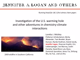
and other adventures in chemistryclimate interactions Loretta J Mickley Pattanun Achakulwisut Becky Alexander Tom Breider Bryan Duncan Rynda Hudman Daniel Jacob ID: 601590
Download Presentation The PPT/PDF document "Investigation of the U.S. warming hole" is the property of its rightful owner. Permission is granted to download and print the materials on this web site for personal, non-commercial use only, and to display it on your personal computer provided you do not modify the materials and that you retain all copyright notices contained in the materials. By downloading content from our website, you accept the terms of this agreement.
Slide1
Investigation of the U.S. warming hole and other adventures in chemistry-climate interactions
Loretta J. MickleyPattanun Achakulwisut, Becky Alexander, Tom Breider, Bryan Duncan, Rynda Hudman, Daniel Jacob, Jennifer Logan, Shannon Koplitz, Eric Leibensperger, Lee Murray, Justin Parrella, David Rind, Lulu Shen, Dominick Spracklen, Amos Tai, Shiliang Wu, Xu Yue, and Lei Zhu
Running head for JAL’s first
atmos
chem paper.
2009 wildfire in Southern CaliforniaSlide2
2013 ~1:1 ratio
1977 1 in 50Slide3
Ozone
PM2.5Millions of people in US living in areas in violation of the EPA standards.What is climate penalty on air quality? How will size of bars change with changing climate?How do trends in short-lived species affect global and regional climate?
Regional
forcings
are as large as global forcings from well-mixed GHGs.Short-lived species can affect methane lifetime.
1990
2001
Calculated trend in surface sulfate
concentrations
Observations in circles
-2 Wm
-2
Leibensperger
et al., 2012Slide4
Atmospheric
ChemistryAssimilated meteorologyGEOS-4GEOS-5
GEOS-
Chem
Atmospheric
C
hemistry
Land cover model
GEOS-
Chem
Meteorology from freely running climate model
Fire prediction model
Chemical feedbacks
Model frameworks
1. Standard
2. Chemistry-climateSlide5
1. Examine observed sensitivities
of short-lived species or other variables to meteorology. E.g. Area burned = f(meteorology)2. Apply sensitivities to archived meteorology from an ensemble of models.Some methods to overcome uncertainties in model apparatus.Yue et al., in review
Area burned (10
5 ha)
R2 ~ 0.5Area burned over Southwest
model
observed
Area burned (10
5
ha)
Timeseries
of area burned
observed
model
3. Benchmark chemistry-climate interactions in the
recent + distant past
with observations.
Arctic 1980-2010
Last Glacial Maximum
Equatorial
Asia 2000s
Area burned in Southwest US may double by 2050.Slide6
Observed US surface temperature trend
GISTEMP 2010 Is the U.S. “warming hole” a signature of cooling due to anthropogenic aerosols? Observed spatial trend in temperatures, 1930-1990No trend between 1930 and 1980.
Warming trend after 1980
Contiguous US
-1
1
0
o
C
1
-1Slide7
We applied decadal trends in anthropogenic aerosol to the GISS climate model.
Increasing sulfate from 1950-1990s. Decreasing sulfate beginning in 1990s.
1950
1960
1970
1980
1990
2001
Leibensperger
et al.,
2012a
Calculated trend in surface sulfate
concentrations
Clearing trend in particles over United States since 1980s suggests possible recent warming.
Circles show observations.Slide8
Leibensperger et al., 2012a.
Direct radiative forcingIndirect radiative forcingForcing from US anthropogenic aerosols peaks in 1980 -1990s.Forcings over Eastern USPeak forcings -2 W m-2, mainly from sulfate.Warming from black carbon offsets the cooling early in the record.
Results suggest little climate benefit to reducing black carbon sources in US.Slide9
C
Leibensperger et al., 2012bCooling from U.S. anthropogenic aerosols during 1970-1990.Results are from two 5-member ensembles, with and without US anthropogenic aerosols.Cooling is greatest over the Eastern US and North Atlantic.1 oC cooling at surface over EastSlide10
D
Model Temperature 1970-1990CD Soil moisture availabilityD Cloud Cover%
%
Cooling over U.S. is not co-located with aerosol burden.Cooling over North Atlantic strengthens Bermuda High, increasing onshore flow of moisture from Gulf of Mexico.
Local changes in cloud cover and soil moisture amplify the cooling effect.Results are controversial.Slide11
Inclusion of US anthropogenic aerosols improves match with observed trends in surface temperatures over the East.
Most of the warming from reducing aerosol sources has already been realized. Results suggest that US anthropogenic aerosols can explain the “warming hole.” Warming since 1990s can be attributed to reductions in aerosol sources. Leibensperger et al., 2012b
Observations
Model without US
aerosols
Standard model
Eastern USSlide12
U.S. BC emissions (
Tg C)1850U.S. SO2 emissions (Tg S)190019502000
BC
SO2
Timeseries of US emissions
How have competing trends in BC and SO2 over 20th century affected regional climate across mid-latitudes?
Ongoing work.
BC aerosol
warms mid- to upper troposphere
cools surface
stabilizes atmosphere
SO
2
cools surface, may augment stabilization.
We will compare model BC with lake core sediments from Adirondacks (Husain et al., 2008)
BC deposition (g m-2 a-1)
1860
1940
obst
observations
model
Deposition in Adirondacks
LeibenspergerSlide13