/
Terrain Analysis Using Digital Elevation Models ( Terrain Analysis Using Digital Elevation Models (

Terrain Analysis Using Digital Elevation Models ( - PowerPoint Presentation

luanne-stotts
luanne-stotts . @luanne-stotts
Follow
415 views
Uploaded On 2016-03-17

Terrain Analysis Using Digital Elevation Models ( - PPT Presentation

TauDEM David Tarboton 1 Dan Watson 2 Rob Wallace 3 1 Utah Water Research Laboratory Utah State University Logan Utah 2 Computer Science Utah State University Logan Utah 3 ID: 259728

core flow cells grid flow core grid cells file elevation ram pit area cluster neighbor quad algebra 0ghz grids

Share:

Link:

Embed:

Download Presentation from below link

Download Presentation The PPT/PDF document "Terrain Analysis Using Digital Elevation..." is the property of its rightful owner. Permission is granted to download and print the materials on this web site for personal, non-commercial use only, and to display it on your personal computer provided you do not modify the materials and that you retain all copyright notices contained in the materials. By downloading content from our website, you accept the terms of this agreement.


Presentation Transcript

Slide1

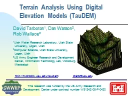
Terrain Analysis Using Digital Elevation Models (TauDEM)

David Tarboton1, Dan Watson2, Rob Wallace31Utah Water Research Laboratory, Utah State University, Logan, Utah 2Computer Science, Utah State University, Logan, Utah3US Army Engineer Research and Development Center, Information Technology Lab, Vicksburg, Mississippi

This research was funded by the US Army Research and Development Center under contract number W9124Z-08-P-0420

http://hydrology.usu.edu/taudem

dtarb@usu.edu

Slide2

Theme

To advance the capability for

hydrologic prediction

by developing

models

that take advantage of new information and process

understanding

enabled by

new technology

Topics

Hydrologic information systems (includes GIS)

Terrain analysis using digital elevation

models(watershed delineation)

Snow hydrology

Hydrologic modelingStreamflow trendsHydrology and Ecology

Research

2Slide3

My Teaching

Physical Hydrology CEE6400 (Fall)GIS in Water Resources CEE6440 (Fall)

A multi-university course presented on-line with shared video in partnership with David Maidment

at the University of Texas at Austin.

Engineering Hydrology CEE3430 (Spring)

Rainfall Runoff Processes (online module)http://www.engineering.usu.edu/dtarb/rrp.htmlSlide4

Deriving hydrologically useful information from Digital Elevation Models

Raw DEM

Pit Removal (Filling)

Flow Field

Channels, Watersheds, Flow Related Terrain Information

Watersheds are the most basic hydrologic landscape elementsSlide5

TauDEM - Channel Network and Watershed Delineation Software

Pit removal (standard flooding approach)

Flow directions and slope

D8 (standard)

D

 (Tarboton, 1997, WRR 33(2):309)

Flat routing (Garbrecht and Martz, 1997, JOH 193:204)

Drainage area (D8 and D

)

Network and watershed delineation

Support area threshold/channel maintenance coefficient (Standard)

Combined area-slope threshold (Montgomery and Dietrich, 1992, Science, 255:826)

Local curvature based (using Peuker and Douglas, 1975, Comput. Graphics Image Proc. 4:375)

Threshold/drainage density selection by stream drop analysis (Tarboton et al., 1991, Hyd. Proc. 5(1):81)

Other Functions: Downslope Influence, Upslope Dependence, Wetness index, distance to streams, Transport limited accumulation

Developed as C++ command line executable functions

MPICH2 used for parallelization (single program multiple data)

Relies on other software for visualization (ArcGIS Toolbox GUI)Slide6

The challenge of increasing Digital Elevation Model (DEM) resolution

1980’s DMA 90 m102 cells/km21990’s USGS DEM 30 m

103 cells/km

2

2000’s NED 10-30 m104 cells/km2

2010’s LIDAR ~1 m

106

cells/km2Slide7

Website and Demohttp://hydrology.usu.edu/taudemSlide8

Model Builder Model to Delineate Watershed using TauDEM toolsSlide9

The starting point: A Grid Digital Elevation Model

Contours

720

700

680

740

680

700

720

740

720

720Slide10

Grid Data Format Assumptions

Input and output grids are uncompressed GeoTIFFMaximum size 4 GBGDAL Nodata tag preferred (if not present, a missing value is assumed)Grids are square (x= y)Grids have identical in extent, cell size and spatial referenceSpatial reference information is not used (no projection on the fly) Slide11

The Pit Removal ProblemDEM creation results in

artificial pits in the landscapeA pit is a set of one or more cells which has no downstream cells around itUnless these pits are removed they become sinks and isolate portions of the watershedPit removal is first thing done with a DEMSlide12

Increase elevation to the pour point elevation until the pit drains to a neighbor

Pit FillingSlide13

Pit Filling

Pits

Pour Points

Original DEM

Pits FilledSlide14
Slide15

Some Algorithm Details

Pit Removal: Planchon Fill Algorithm

Initialization

1

st

Pass

2

nd

Pass

Planchon

, O., and F.

Darboux

(2001), A fast, simple and versatile algorithm to fill the depressions of digital elevation models,

Catena

(46), 159-176.Slide16

Parallel Approach

MPI, distributed memory paradigmRow oriented slicesEach process includes one buffer row on either sideEach process does not change buffer rowSlide17

Parallel Scheme

Communicate

Initialize( Z,F)

Do

for all grid cells

i

if

Z(

i

) > n

F(

i

) ← Z(

i

)

Else

F(

i

) ← n

i

on stack for next pass

endfor

Send(

topRow

, rank-1 )

Send(

bottomRow

, rank+1 )

Recv

(

rowBelow

, rank+1 )

Recv

(

rowAbove

, rank-1 )

Until F is not modified

Z denotes the original elevation.

F denotes the pit filled elevation.

n denotes lowest neighboring elevation

i

denotes the cell being evaluated

Iterate only over stack of changeable cells Slide18

80

74

63

69

6756

60

52

48

30

4

5

6

3

7

2

1

8

D8 Flow Direction Model

- Direction of steepest descent

Slope = Drop/Distance

Steepest down slope directionSlide19

Grid NetworkSlide20

1

1

1

1

1

1

1

2

1

1

1

1

1

1

3

3

3

11

2

1

2

5

15

20

2

The area draining each grid cell includes the grid cell

itself.

1

1

1

1

1

1

1

2

1

1

1

1

1

1

3

3

3

11

2

1

5

2

2

20

15

Contributing Area (Flow Accumulation)Slide21

1

1

1

1

1

1

1

2

1

1

1

1

1

1

3

3

3

11

2

1

2

5

15

20

2

Flow Accumulation

> 10 Cell Threshold

1

1

1

1

1

1

1

2

1

1

1

1

1

1

3

3

3

2

1

5

2

2

11

15

20

Stream Network for 10 cell

Threshold Drainage Area

Stream DefinitionSlide22

Watershed Draining to OutletSlide23

Watershed and Stream GridsSlide24

DEM Delineated Catchments and Stream NetworksFor every stream segment, there is a corresponding

catchmentCatchments are a tessellation of the landscape Based on the D8 flow direction modelSlide25

Edge contamination

Edge contamination arises due to the possibility that a contributing area value may be underestimated due to grid cells outside of the domain not being counted. This occurs when drainage is inwards from the boundaries or areas with no data values. The algorithm recognizes this and reports "no data" resulting in streaks of "no data" values extending inwards from boundaries along flow paths that enter the domain at a boundary. Slide26

D

Representation

of Flow Field

D

8

67

56

52

48

Steepest single direction

Tarboton, D. G., (1997), "A New Method for the Determination of Flow Directions and Contributing Areas in Grid Digital Elevation Models," Water Resources Research, 33(2): 309-319.)Slide27

D-Infinity Slope, Flow Direction and Contributing AreaSlide28

Pseudocode for Recursive Flow Accumulation

Global P, w, A, FlowAccumulation

(i)

for all k neighbors of i

if Pki>0

FlowAccumulation(k)

next k

return

P

kiSlide29

General Pseudocode

Upstream Flow Algebra Evaluation

P

ki

Global

P

,

,

FlowAlgebra

(

i

)

for all k neighbors of

i

if

P

ki

>0

FlowAlgebra

(k)

next k

i

= FA(

i

,

P

ki

,

k

,

k

)

returnSlide30

Example: Retention limited runoff generation with run-on

Global

P

,

(

r

,

c

)

,

q

FlowAlgebra

(

i

)

for all k neighbors of

i

if

P

ki

>0

FlowAlgebra

(k)

next k

return

r

c

q

i

q

kSlide31

0.6

0.4

1

A

B

C

D

r=7

c=4

q=3

r=5

c=6

q

in

=1.8

q=0.8

r=4

c=6

q=0

1

r=4

c=5

q

in

=2

q=1

Retention Capacity

Runoff from uniform input of 0.25

Retention limited runoff with run-onSlide32

Useful for a tracking contaminant or compound subject to decay or attenuationSlide33

Supply

Capacity

Transport

Deposition

2

2

)

tan(

b

T

cap

c

a

=

å

+

=

}

,

min{

cap

in

out

T

T

S

T

å

-

+

=

out

in

T

T

S

D

Transport limited accumulation

Useful for modeling erosion and sediment delivery, the spatial dependence of sediment delivery ratio and contaminant that adheres to sediment

SSlide34

A=1

A=1

A=1

A=1.5

A=3

A=1.5

A=1

D=2

D=1

A=1

D=1

D=1

B=-2

Queue’s empty so exchange border info.

B=-1

A=1

A=1

A=1

D=0

A=3

A=1.5

A=1

D=2

D=1

A=1

D=1

D=1

B=-2

A=1

A=1

A=1

A=1.5

A=3

A=1.5

A=1

D=0

D=0

A=1

D=1

D=1

resulting in new D=0 cells on queue

A=1

A=1

A=1

A=1.5

A=3

A=1.5

A=1

A=5.5

A=2.5

A=1

A=6

A=3.5

and so on until completion

A=1

A=1

A=1

D=0

D=0

D=0

A=1

D=2

D=1

A=1

D=1

D=1

D=0

D=0

D=0

D=1

D=3

D=1

D=0

D=2

D=1

D=0

D=3

D=1

A=1

D=0

D=0

D=1

D=2

D=0

A=1

D=2

D=1

D=0

D=2

D=1

A=1

A=1

D=0

D=1

D=1

D=0

A=1

D=2

D=1

A=1

D=1

D=1

A=1

A=1

A=1

D=1

D=0

A=1.5

A=1

D=2

D=1

A=1

D=1

D=1

B=-1

Decrease cross partition dependency

Parallelization of Contributing Area/Flow Algebra

Executed by every process with grid flow field P, grid dependencies D initialized to 0 and an empty queue Q.

FindDependencies

(P,Q,D)

for all

i

for all k neighbors of

i

if

P

ki

>0

D(

i

)=D(

i

)+1

if

D(

i

)=

0

add

i

to Q

next

Executed by every process with D and Q initialized from

FindDependencies

.

FlowAlgebra

(P,Q,D,

,

)

while Q isn’t empty

get

i

from Q

i

= FA(

i

,

P

ki

,

k

,

k

)

for each

downslope

neighbor n of

i

if P

in

>0

D(n)=D(n)-1

if D(n)=0

add n to Q

next n

end while

swap process buffers and repeat

1. Dependency grid

2. Flow algebra functionSlide35

Capability to run larger problems


Processors

used

Grid size

Theoretcal

limit

Largest run

2008

TauDEM

4

1

0.22 GB

0.22 GB

Sept 2009

Partial

implement-

ation

8

4 GB

1.6 GB

June 2010

TauDEM

5

8

4 GB

4 GB

Sept 2010

Multifile

on 48 GB RAM PC

4

Hardware limits

6 GB

Sept 2010

Multifile

on

cluster with 128 GB RAM

128

Hardware limits

11 GB

1.6 GB

0.22 GB

4 GB

6 GB

11 GB

At 10 m grid cell size

Single file size limit 4GB

Capabilities SummarySlide36

Parallel Pit Remove timing for NEDB test dataset (14849 x 27174 cells

1.6 GB).

128 processor cluster

16 diskless Dell SC1435 compute nodes, each with 2.0GHz dual quad-core AMD

Opteron

2350 processors with 8GB RAM

8 processor PC

Dual quad-core Xeon E5405 2.0GHz PC with 16GB RAM

Improved runtime efficiencySlide37

Parallel D-Infinity Contributing Area Timing for Boise River dataset (24856 x 24000 cells ~ 2.4 GB)

128 processor cluster 16 diskless Dell SC1435 compute nodes, each with 2.0GHz dual quad-core AMD Opteron

2350 processors with 8GB RAM

8 processor PCDual quad-core Xeon E5405 2.0GHz PC with 16GB RAM

Improved runtime efficiencySlide38

Dataset

Size

Hardware

Number of Processors

PitRemove

(run time seconds)

D8FlowDir

(run time seconds)


(GB)


Compute

Total

Compute

Total

GSL100

0.12

Owl (PC)

8

10

12

356

358

GSL100

0.12

Rex (Cluster)

8

28

360

1075

1323

GSL100

0.12

Rex (Cluster)

64

10

256

198

430

GSL100

0.12

Mac

8

20

20

803

806 

YellowStone

2.14

Owl (PC)

8

529

681

4363

4571

YellowStone

2.14

Rex (Cluster)

64

140

3759

2855

11385

Boise River

4

Owl (PC)

8

4818

6225

10558

11599

Boise River

4

Virtual (PC)

4

1502

2120

10658

11191

Bear/Jordan/Weber

6

Virtual (PC)

4

4780

5695

36569

37098

Chesapeake

11.3

Rex (Cluster)

64

702

24045


Owl is an 8 core PC (Dual quad-core Xeon E5405 2.0GHz) with 16GB RAM

Rex is a 128 core cluster of

16 diskless Dell SC1435 compute nodes, each with 2.0GHz dual quad-core AMD

Opteron

2350 processors with 8GB RAM

Virtual is a virtual PC resourced with 48 GB RAM and 4 Intel Xeon E5450 3 GHz processors

Mac is an 8 core (Dual quad-core Intel Xeon E5620 2.26 GHz) with 16GB RAM

Scaling of run times to large gridsSlide39

Owl is an 8 core PC (Dual quad-core Xeon E5405 2.0GHz) with 16GB RAM

Rex is a 128 core cluster of 16 diskless Dell SC1435 compute nodes, each with 2.0GHz dual quad-core AMD Opteron 2350 processors with 8GB RAM Virtual is a virtual PC resourced with 48 GB RAM and 4 Intel Xeon E5450 3 GHz processors

Scaling of run times to large gridsSlide40

ProgrammingC++ Command Line Executables that use MPICH2ArcGIS Python Script Tools

Python validation code to provide file name defaultsShared as ArcGIS ToolboxSlide41

while(!que.empty()) {

//Takes next node with no contributing neighbors

temp = que.front(); que.pop

();

i

=

temp.x

;

j =

temp.y

;

// FLOW ALGEBRA EXPRESSION EVALUATION

if(flowData->isInPartition(i,j)){

float

areares

=0

.;

//

initialize the result

for

(k=1

; k<=8; k++)

{

// For each neighbor

in

= i+d1[k

];

jn

= j+d2[k];

flowData->getData(in,jn

, angle); p

= prop(angle, (k+4)%8); if

(p>0.){ if

(areadinf->isNodata(

in,jn))con=true;

else{

areares=areares+p*

areadinf->getData(in,jn,tempFloat);

}

} }

}

// Local inputs

areares

=areares+dx;

if(con &&

contcheck==1)

areadinf->setToNodata(

i,j);

else

areadinf

-

>

setData

(

i,j,areares

);

//

END FLOW ALGEBRA EXPRESSION EVALUATION

}

Q based block of code to evaluate any “flow algebra expression”Slide42

while

(!finished) { //Loop within partition while(!

que.empty())

{ .... // FLOW ALGEBRA EXPRESSION EVALUATION

}

// Decrement neighbor dependence of downslope cell

flowData-

>getData

(

i

, j, angle);

for

(k=1

; k<=8; k++) {

p = prop(angle, k); if(p>0.0) { in = i+d1[k]; jn = j+d2[k];

//

Decrement the number of contributing neighbors in neighbor

neighbor-

>

addToData

(

in,jn

,(

short

)-1);

//

Check if neighbor needs to be added to

que

if

(

flowData

-

>

isInPartition

(in,jn) && neighbor->getData(in, jn

, tempShort) == 0 ){ temp.x

=in; temp.y=jn;

que.push(temp);

} }

}}

//Pass information across partitions

areadinf->share();neighbor-

>addBorders();Maintaining to do Q and partition sharingSlide43

Python Script to Call Command Linempiexec

–n 8 pitremove –z Logan.tif –fel Loganfel.tifSlide44

PitRemoveSlide45

Validation code to add default file namesSlide46

Multi-File approachTo overcome 4 GB file size limitTo avoid bottleneck of parallel reads to network files

What was a file input to TauDEM is now a folder inputAll files in the folder tiled together to form large logical gridSlide47

Processor Specific Multi-File Strategy

Core 1Core 2

Shared file store

Node 2 local disk

Node 1 local disk

Core 1

Core 2

Node 2 local disk

Node 1 local disk

Output

Shared file store

Input

Scatter all input files to all nodes

Gather partial output from each node to form complete output on shared storeSlide48

Summary and ConclusionsParallelization speeds up processing and partitioned processing reduces size limitations

Parallel logic developed for general recursive flow accumulation methodology (flow algebra) Documented ArcGIS Toolbox Graphical User Interface32 and 64 bit versions (but 32 bit version limited by inherent 32 bit operating system memory limitations)PC, Mac and Linux/Unix capabilityCapability to process large grids efficiently increased from 0.22 GB upper limit pre-project to where < 4GB grids can be processed in the ArcGIS Toolbox version on a PC within a day and up to 11 GB has been processed on a distributed cluster (a 50 fold size increase) Slide49

Limitations and Dependencies

Uses MPICH2 library from Argonne National Laboratory http://www.mcs.anl.gov/research/projects/mpich2/ TIFF (GeoTIFF) 4 GB file size (for single file version)Run multifile version from command line for > 4 GB datasetsProcessor memory