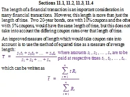
PPT-The length of a financial transaction is an important consi PowerPoint Presentation

Sections 111 112 113 114 An improved measure of length which would take coupon rate into account is to use the method of equated time as a measure of average length

Upload by luanne-stotts
Published on 2016-04-07

Presentation Embed Code

<iframe width="560" height="315" src="https://www.docslides.com/embed/275986" frameborder="0" allowfullscreen></iframe>

Download Presentation

Download Presentation The PPT/PDF document "The length of a financial transaction is..." is the property of its rightful owner. Permission is granted to download and print the materials on this web site for personal, non-commercial use only, and to display it on your personal computer provided you do not modify the materials and that you retain all copyright notices contained in the materials. By downloading content from our website, you accept the terms of this agreement.