ISPRS Workshop on Updating Geospatial Database s with - PDF document

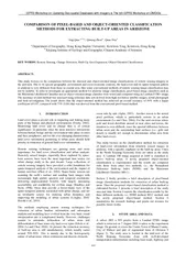
ISPRS Workshop on Updating Geo-spatial Databases with Imagery & The 5th ISPRS Workshop on DMGISs COMPARISON OF PIXEL-BASED AND OBJECT-ORIENTED CLASSIFICATION ILT-UP AREAS IN ARIDZONE *, Qiming Zhou , Quan HouDepartment of Geography, Hong Kong Baptist University, Kowloon Tong, Kowloon, Hong Kong Xinjiang Institute of Ecology and Geography, Chinese Academy of Sciences ISPRS Workshop on Updating Geo-spatial Databases with Imagery & The 5th ISPRS Workshop on DMGISs railway lines. With increasingly intensifying social and economic development, the local ecological environment has changed dramatically. This study area is one of the regions with the most developed economy in Xinjiang and represents a miniature of the economic development in north Xinjiang. The ETM image was geometrically corrected and registered on the map coordinates using image-to-image registration to the master SPOT image of 2002 (come from National Fundamental Geographic Information Center). A total of 37 Ground Control Points (GCPs) were used, which resulted in an RMS error of less than 0.5 pixels. A set of ortho-corrected aerial photos acquired in 2000 is used as reference data. Figure 1. ETM image of the study area. (E to E longitude; N to N latitude. Combination of band 4, 3, 2. Collected on 7 August 2000.) Figure 2. Map of the study area: the Centre Town of Manas County, City of Shihezi and part of regimental farm of Division 8, at North Xinjiang Economic Zone, China THE LAND COVER FEATURES OF REMOTE SENSING IN ARID AREA From the point of view of landscape ecology, the arid region can be deemed as a special combination of mountains, oases, and desert. The study area is a representative oasis region. Oases typically stretch along rivers, which is the case in this study region. The Manas river in the study region slows down after running out from the mountain, and the sediment carried by the river deposits, which finally forms gradual alluvial fans. The riverbed mainly contains gravels, and is easily to leak out water. Along the riverside are cities and towns surrounded by irrigated agricultural land. Different features usually show different characteristics in remote sensing images, which enables interpreting features from images. The image characteristics useful in image interpretation include shape, size, colour, tone, shadow, location, and texture. These characteristics make the keys for image interpretation. The following table shows the characteristics of major landscape types in the study area (Table 1). PIXEL-BASED AND OBJECT-BASED IAMGE CLASSIFIERS Image classification refers to the extraction of differentiated classes or themes, usually land-cover and land-use categories, from raw remotely sensed digital satellite data. The information contained in a remotely sensed image and can be used to conduct image classification includes spectral pattern, spatial pattern and temporal pattern. Spectral pattern is the combination of digital numbers (DNs) for different feature types. Spatial pattern refers to the spatial relationship of the pixels, such as image texture, pixel proximity, feature size, and shape. Temporal pattern refers to temporal characteristics of the features. A wide range of classification methods has been developed to derive land cover information from remotely sensed images. Since remotely sensed images consist of rows and columns of pixels, per-pixel approach, either supervised or un-supervised, has been the conventional method for land cover mapping (Dean and Smith, 2003). Pixel-based classification methods, by using multi-spectral classification techniques, assign a pixel to a class fundamentally according to the spectral similarities (Jensen, 1986; Gong et al., 1992; Casals-Carrasco et al., 2000). Although the techniques are well developed and many successful applications have been reported, it suffers from ignoring the spatial pattern in classification. The Maximum Likelihood classification (MLC), which is the most widely used per-pixel method, is argued to be limited by utilizing only spectral information without considering texture and contextual information (Zhou and Robson, 2001; Dean and Smith, 2003). Unlike traditional pixel-based methods, an object-oriented method treats the image as a set of meaningful objects rather than single pixels (Giada et al., 2003; Gao et al.segmentation is a preliminary step in object-oriented image classification. Then the spatial information of the segmented parcels can be derived and employed in further image analysis. The enrichment of the information used in image classification is expected to improve classification accuracy (Gao et al.2006). Recent experiments show that landscape metrics, which are measures of spatial pattern for the segmented parcels from landscape ecology point of view, can be a useful tool in remote sensing image classification, especially when the features of ISPRS Workshop on Updating Geo-spatial Databases with Imagery & The 5th ISPRS Workshop on DMGISs interest have similar spectral properties but differing shape or spatial properties (Frohn, 1998; 2006). For example, a perimeter-to-area shape complexity metric called the Square Pixel Metric (SqP) is used in differentiating lakes from rivers, classification of drained basins, and classification of natural vs. anthropogenic pastures, with all practice yielding an overall accuracy over 90% (Frohn, 2006). This research proposed an objeccation method for the arid region with an emphasis on delineation of built-up areas. Following the common practice of comparing image classification methods (e.g., Zha et al., 2003; Erbek et al.2004), the result of this method will be compared with the conventional MLC method. In addition, a recently proposed NDBI method (Zha et al., 2003), which is developed dedicatedly to automate the process of mapping built-up areas, is also selected as a test-bed, so as to highlight the performance of the proposed object-based classification method to derive built-up areas. Normalized Difference Built-up Index (NDBI, pixel-based) The NDBI method is proposed aiming to automate the process of mapping built-up areas. It makes use of both the conventional Normalized Difference Vegetation Index (NDVI) measurement and the newly proposed Normalized Difference Built-up Index (NDBI). A classification of Landsat TM image of Nanjing, China yields an overall accuracy of 92.6%, which is claimed as superior to a common MLC method (Zha et al.2003). Beyond its high-standard performance in terms of classification accuracy, the NDBI method, as a decision tree s non-parametric nature, and several attractive properties of simplicity, flexibility, and computational efficiency (Friedl and Brodley, 1997). The non-parametric property means that non-normal, non-homogenous and noisy data sets can be handled. In addition, a decision tree classifier has a simple form, and thus can be stored compactly and re-used for new data sets. The simple tree structure also provides easy interpretation of the classified themes. 4545TMTMTMTMNDBI (1) Three category were extracted form the NDBI: build-up area & barren soil, water body, vegetation. The results are shown as Figure 3 and Figure 4. Maximum Likelihood Classification (MLC, pixel-based) fication is a classical classifier and the most common technique presented in the literature (Benedictsson et al., 1990; Foody et al., 1992; Paola, 1994). The maximum likelihood decision rule is based on the probability that a pixel belongs to a particular class. The basic equation assumes that these probabilities are equal for all classes, and that the input bands have normal distributions. Pixel-based supervised maximum likelihood image classification was performed in ERDAS 8.5. Referring to the land use and land cover classification system et al., 1976) and landscape type, In this study nine land cover categories were classified, which are: (1) build-up area: mixed urban, settlement or built up land; (2) cropland: cropland or fallow; (3) garden plot: orchards, vineyards or nurseries; (4) sparse woodland: low coverage mixed shrub, desert scrub or bare ground; (5) dense woodland: high coverage mixed shrub or shelter belt; (6) grassland: pasture or desert grass; (7) river flat: dry river bed or river flat; (8). water body: reservoir or fish pond. It is important that training samples be representative of the class that you are trying to identify. With the help of aerial photos and field work investigation, knowledge of the data, and of the classes desired, have been acquired before classification. Training samples (a set of pixels) of represent patterns and land cover features recognized can be selected more determinately. Samples are selected elaborately and the Seed Properties dialog and AOI tools can be used. The seed pixel is used as a model pixel, against which the pixels that are contiguous to it are compared based on parameters (Neighbourhood, Geographic Constraints, Spectral Euclidean Distance) specified by user. Using the signature separability analysis, Bands 3, 4and 5 were used. Signature separability is a statistical measure of distance between two signatures. Separability can be calculated for any combination of bands that is used in the classification. For the distance (Euclidean) evaluation, the spectral distance between the mean vectors of each pair of signatures is computed. If the spectral distance between two samples is not significant for any pair of bands, then they may not be distinct enough to produce a successful classification. The spectral distance is also the basis of the minimum distance classification. Therefore, computing the distances between signatures can help to predict the results of a minimum distance classification. Object-Oriented Image Analysis Object-oriented classification does not operate directly on single pixels, but image objects which refer to homogeneous, spatially contiguous regions obtained by dividing image, namely image segmentation. Image segmentation is a preliminary step in object-oriented image classification, and the segmentation technique can be grouped into three types: thresholding/clustering, region based, and edge based (Fu and Mui, 1981; Haralick and Shapiro, 1985). The region-growing method is the one most widely applied in programs. More information about image segmentation techniques can be found in Fu and Mui (1981), Haralick and Shapiro (1985), and Pal The accuracy of segmentation directly influences the performance of object-oriented image classification. Only good segmentation results can lead to object-oriented image classification out-performing pixel-based classification. Human interpretation and correction is considered as the best way to evaluate the segmentation output (Pal and Pal, 1993), and some methods have been developed to quantitatively measure the degree of over-and under segmentation of regions, and to measure the discrepancy between the positions of the region After the image objects are generated, many methods can be used to classify them. The simple classification can conducted only by comparing the mean grey values of the objects with those of the training samples, those objects are classified to the classes to which they are most close. And the advanced classification will combine ancillary data, such as shape characteristics and neighbourhood relationships (Shackelford and Davis, 2003; Walter, 2004) extracted from the image objects, with spectral information. ISPRS Workshop on Updating Geo-spatial Databases with Imagery & The 5th ISPRS Workshop on DMGISs Image Landscape type Color, tone, and texture Location land-cover 1 Plain farmland Block or strip shaped, Between mountain and desert, along river or irrigation channel Clump (separate or linked), Plantation\Garden Clump, green Sparsely distributed in econoOic forest 3 City and town Clump, gray-blue, scattered with red Alluvial fans Settlement 4 headquarter Clump, gray-blue Scattered in the oasis Scattered regiand villages 5 Industrial and Clump and points, black or dark gray In front of mountain Mega-project and mining site 6 High coverage Clump, red Low mountain Mainly shrub, high coverage 7 Low coverage Gray-blue scattered with faint red clumpsAt low mountain, in the margin of artificial oasis Mainly southernwood, low coverage Vegetation in Strip, gray-blue At the upper part of the alluvial fans in front of Vegetation in desert, very low coverage River flat Gray-blue At ground water leakage belt, downward the site river runs out mountain River flat gravel, sands 10 Water body Block, blue or dark Water source and reservoir River, lake, and reservoir Table 1. The characteristics of major landscape types in Arid Area Based on RS Images Object-oriented classification was performed in eCognition, which is an object based processing software program made available in 2000 from Definiens Imaging GmbH and was claimed to be user-friendly, multi-scaled, and fully functional (Blaschke and Strobl, 2001). Image segmentation in eCognition is a multi-resolution, bottom up, region-merging technique starting with one-pixel objects. Image objects are extracted from the image in a number of hierarchical segmentation levels, and each subsequent level yields image objects of a larger average size by combining objects from a level below, which represents image information on different scales simultaneously. Objects are grouped into a larger object based on spectral similarity, contrast with neighbouring objects, and shape characteristics of the resulting object. These three characteristics are grouped into a single parameter called heterogeneity. With a certain ‘scale’ parameter, three criteria define the heterogeneity of the objects: colour, smoothness, and compactness, the last two being known as shape criterion. Colour criterion defines the weight the spectral values of the image layers contribute to the entire homogeneity criterion, as opposed to the weight the shape homogeneity. Maximum colour criterion 1.0 results in objects spatially most homogeneous; however it can not have a value less than 0.1 because of without spectral information the created objects would not be related to the spectral information at all. Smoothness is to optimize image objects with regard to smooth borders and compactness with regard to compact objects, which should be used when different image objects rather compact, but separated from non-compact objects only by a relatively weak contrast, are to be extracted (Baatz , 2004). The classifier of object-oriented image classification is nearest neighbour, which is a soft classifier, based on fuzzy logic. The nearest neighbour classifier classifies image objects in a given feature space with given samples for the classes of concern. Firstly, sample objects are declared for each class, then the algorithm searches for the closest sample object in the feature space for each image object. All class assignments in eCognition are determined by assignment values in the range 0–1. The closer an image object is located in the feature space to a sample of a class, the higher the membership degree to this class. The best classification result keeps the highest membership values (Definiens Imaging GmbH, 2002; Baatz et , 2004). The methodology flowchart of object oriented image analysis is shown in Figure 3. Accuracy Assessment Spatial data accuracy concerns two aspects, i.e., positional accuracy and thematic accuracy. Particularly for remote sensing data, positional accuracy refers to the accuracy of a geometrically rectified image, while for remote sensing classifications, thematic accuracy is often termed classification accuracy (Janssen and van der Wel, 1994). To adequately ascribe uncertainty, or in other words, to assess the accuracy, in maps derived from remotely sensed images has been one of the most outstanding challenges related to uncertainty in remote sensing. The analysis and estimation protocols used to analyze the reference sample data constitute the final component of an accuracy assessment. Up to date, an error matrix, or sometimes-called confusion matrix or contingency table, has been the core of the analysis and estimation procedures for an accuracy assessment (Stehman and Czaplewski, 1998). ISPRS Workshop on Updating Geo-spatial Databases with Imagery & The 5th ISPRS Workshop on DMGISs Confusion matrix is a simple cross-tabulation of the mapped class label against that observed in the ground or reference data for a sample of cases at specified locations. The overall accuracy is calculated by dividing the number of correctly classified pixels (presented as entries in the major diagonal of the confusion matrix) by the total number of reference pixels. Though simple, the overall accuracy has been the most conventional approach accuracy assessment (Woodcock, 2002). An improvement to this overall accuracy assessment metric is Figure 3. The methodology flowchart of object oriented image analysis the Kappa coefficient of agreement, which expresses the proportionate reduction in error generated by a classifier compared with the error of a completely random classification. Beyond the compensation for chance agreement, the Kappa coefficient can be used in the z-test of the significance of the difference between two coefficients, thus enables a comparison between different classifications in terms of accuracy. Sampling design is of critical importance for accuracy assessment, since all further explorations are based on the sample data. A wide range of designs has been proposed. Among them, the most basic and commonly applied ones are simple random sampling (SRS), systematic sampling, stratified sampling, and cluster sampling. In my study stratified random sampling was adopted. Samples are randomly generated, and then labelled by referring to the ortho-corrected aerial photos. Totally 900 reference sites are selected as ground reference RESULTS AND DISCUSSION The classification result of the NDBI method is shown in figure 4. Clearly the performance is poor, especially in terms of delineating built-up area from surrounding features in the arid environment. The sparse woodland, bare ground and dry riverbed are categorized into the same land-cover class with built-up area. The NDBI method, which makes use only spectral patterns, is unable to differentiate urban areas from barren (e.g. sandy beaches) because of their similarity in spectral response. Thus the reliability of this method is severely damaged in mapping peripheral urban areas where barren or fallow land is widespread, which is a common situation in arid Figure 2 also shows the classified images using MLC and object-oriented method. Clearly, the sparse woodland, bare ground and dry riverbed can be visually identified from the classified images, indicating that these two methods can somehow differentiate built-up areas from it background features. The accuracy assessment of these two classifiers can be found in table 2 and table 3. The MLC method yields an overall accuracy of 70.89%, which is much lower than the objective set by Anderson et al. (1976). A closer examination of the error matrix reveals that major confusion occurs in the following pairs of land-cover types: sparse woodland vs. grassland, cropland vs. dense woodland, garden vs. dense woodland, water vs. dense woodland, and built-up area vs. dense woodland. The kappa coefficient, which is 0.6633, is quite low too, indicating the MLC method is still an unsatisfactory one to classify remotely sensed images of the arid regions. The object-oriented classifier outruns the other two classifiers in both overall accuracy and class-based accuracy. The overall accuracy reaches 89.33%, surpassing the objective set by et al. (1976). The kappa coefficient, which is 0.8773, is quite high too, especially for a classification containing as many as eight types of land-covers. In addition, the object-oriented method significantly narrowed down the variation of class-based accuracies compared with the result by the MLC method. Thus it meets the requirement that the accuracy of interpretation for the different categories should be about equal et al., 1976). In particular, relatively high accuracy for built-up area, both producer’s one and user’s one, is achieved by the object-oriented approach. The producer’s accuracy and user’s accuracy for built-up area by the object-oriented method are 84.76% and 76.07%, respectively. Whilst the corresponding producer’s accuracy and user’s accuracy by the MLC method are 72.65% and 68.55%. Obviously the object-oriented is more reliable to delineate built-up areas. ETM image Image segmentation Object oriented image analysis Building knowledge base Referring aerial photos Classify image with Nearest Neighbour (NN) classifier Training samples selection Classified image in eCognition Accuracy assessment ISPRS Workshop on Updating Geo-spatial Databases with Imagery & The 5th ISPRS Workshop on DMGISs Figure 4. Landsat image and classification result Up-left: Landsat TM image of 7 August 2000. RGB = TM 4, 5, 3 Up-right: Classification result of the NDBI method Bottom-left: Classification result of maximum likelihood classifier Bottom-right: Classification result of object-oriented method ISPRS Workshop on Updating Geo-spatial Databases with Imagery & The 5th ISPRS Workshop on DMGISs Reference Data Classified Data 1 2 3 4 5 6 7 8 Classified Reference AccuracyAccuracy Water body 57 2 1 0 0 0 0 0 60 91 57 62.64% 95.00% 0.9444 Bottomland 8 95 3 1 0 0 0 0 107 103 95 92.23% 88.79% 0.8734 Build-up area 4 5 85 11 12 3 4 0 124 117 85 72.65% 68.55% 0.6385 Sparse woodland 2 0 5 92 14 4 23 1 141 109 92 84.40% 65.25% 0.6046 Cropland 0 0 2 1 1263 0 39 171 189 126 66.67% 73.68% 0.6669 Garden 0 0 0 0 0 49 0 0 49 90 49 54.44% 100.00% 1.0000 Grassland 0 0 1 4 0 2 59 0 66 86 59 68.60% 89.39% 0.8827 Dense woodland 20 1 20 0 37 29 0 75 182 115 75 65.22% 41.21% 0.3260 Column Total 91 103 11710918990 86 115900 900 638 Overall Classification Accuracy = 70.89% Overall Kappa Statistics = 0.6633 Table 3. Error matrix of image classification by maximum likelihood classifier Reference Data Classified Data Classified Reference Accuracy Accuracy Water body 95 4 3 0 1 1 1 0 105 99 95 95.96% 90.48% 0.8930 Bottomland 0 100 0 0 0 0 0 0 100 107 100 93.46% 100.00% 1.0000 Build-up area 2 0 89 0 3 1 17 5 117 105 89 84.76% 76.07% 0.7291 Sparse woodland 0 1 3 1041 0 0 0 109 107 104 97.20% 95.41% 0.9479 Cropland 0 0 2 1 0 1 1522 158 198 152 76.77% 96.20% 0.9513 Garden 0 2 1 0 2 0 12 85 102 95 85 89.47% 83.33% 0.8137 Grassland 0 0 7 2 0 88 3 0 100 91 88 96.70% 88.00% 0.8665 Dense woodland 2 0 0 0 91 0 13 3 109 98 91 92.86% 83.49% 0.8147 Column Total 99 107 10510798 91 19895 900 900 804 Overall Classification Accuracy = 89.33% Overall Kappa Statistics = 0.8773 Table 4. Error matrix of image classification by object-oriented image classifier ISPRS Workshop on Updating Geo-spatial Databases with Imagery & The 5th ISPRS Workshop on DMGISs CONCLUSIONS The NDBI method is found to be unable to differentiate urban areas from the background features such as sparse woodland, bare ground and dry riverbed in arid regions. The usability of such a pixel-based spectral classifier is severely limited in the arid regions mainly due to the common presence of land-covers of bare ground and dry riverbed, which have similar spectral response with built-up areas. The object-oriented classifier outruns the MLC method overwhelmingly. It yields an overall accuracy of 89.33%, whereas the overall accuracy for the MLC method is only 70.89%. The variation between accuracies of different classes is significantly narrowed down in the object-orient classification. In particular, the object-orient approach also has superior performance in classifying built-up area. The object-oriented classification also has disadvantages although it outperforms the pixel-based one. Firstly, the classification accuracy depends on the quality of image segmentation. If objects are extracted inaccurately, subsequent classification accuracy will not improve. Secondly, classification error could be accumulated due to the error in both image segmentation and classification process. Thirdly, once an object is misclassified, all pixels in this object will be misclassified. Finally, the derived features from objects sometimes may add more useful information to solve the flectance on pixels, they also can may add misinformation, which usually results in poor classification performance. These flaws remain as possible directions for future research efforts on the object-oriented REFERENCES Anderson, J. R., E. E. Hardy, J. T. Roach, and R. E. Witmer. A land use and land cover classification system for use with remote sensor data. Washington, DC: US Geological Survey. Aplin, P. 2003. Comparison of simulated IKONOS and SPOT HRV imagery for classifying urban areas. In Remotely Sensed , edited by Victor Mesev. London and New York: Taylor & Francis. pp. 23-45. Baatz, M. and A. Schape. 2000. Multiresolution segmentation - an optimization approach for high quality multi-scale image segmentation. In Angewandte Geographische Informations - Verarbeitung XII,, eds. J. Strobl, T. Blaschke and G. Griesebner, 12–23. Karlsruhe: Wichmann Verlag. Benedictsson, J. A., P. H. Swain, and O. K. Ersoy. 1990. Neural network approaches versus statistical methods in classification of multisource remote sensing data. Transactions on Geoscience and Remote Sensing 28, (4): 540–Blaschke, T. and J. Strobl. 2001. What’s wrong with pixels? Some recent development interfacing remote sensing and GIS. 14, (6): 12–17. Casals-Carrasco, P., S. Kubo, and B. Babu Madhavan. 2000. Application of spectral mixture analysis for terrain evaluation International Journal of Remote Sensing 21, Dean, A. M., and G. M. Smith. 2003. An evaluation of per-parcel land cover mapping using maximum likelihood class International Journal of Remote Sensing 24, (14): Definiens Imaging Gmbh. 2002. eCognition User Guide: Multiresolution Segmentation. Available online at: www.definiens-imaging.com/course/03_segmentation%20I/1segmentation_I.htm (accessed 19 February 2002). Erbek, Sunar F., C. Ozkan, and M. Taberner. 2004. Comparison of maximum likelisupervised artificial neural activities. International Journal of Remote Sensing 25, (9)(May): 1733-1748. Foody, G. M., N. A. Campbell, N. M. Trood, and T. F. Wood. 1992. Derivation and application of probabilistic measures of class membership from the maximum likelihood classification. Photogrammetric Engineering & Remote Sensing 58, (9): Friedl, M. A., and C. E. Brodley. 1997. Decision tree classification of land cover from remotely sensed data. Remote Sensing of Environment 61, (3) (September): 399-409. Frohn, Robert C. 1998. Remote sensing for landscape ecology: new metric indicators for the monitoring, modeling, and assessment of ecosystems. Boca Raton, FL: Lewis Publishers. Frohn, Robert C. 2006. The use of landscape pattern metrics in remote sensing image classification. International Journal of 27, (10)(May): 2025-2032. Fu, M. and C. Mui. 1981. A survey on image segmentation. Pattern RecognitionGao, Yan, J. F. Mas, B. H. P. Maathuis, Xiangmin Zhang, and P. M. Van Dijk. 2006. Comparison of pixel-based and object-oriented image classification approaches - a case study in a coal fire area, Wuda, Inner Mongolia, China. International Journal 27, (18)(September): 4039-4055. Giada, S., T. De Groeve, D. Ehrlich, and P. Soille. 2003. Information extraction from very high resolution satellite imagery over Lukole refugee camp, Tanzania. International Journal of Remote Sensing 24, (22)(November): 4251-4266. Gong, P., D. Marceau, and P. J. Howarth. 1992. A comparison of spatial feature extraction algorithms for land use classification with SPOT HRV data. Remote Sensing of EnvironmentHaralick, R. M. and L. G. Shapiro. 1985. Image segmentation techniques. Computer Vision Graphics and Image Processing29, 100-132. Herold, Martin, Noah C. Goldstein, and Keith C. Clarke. 2003. The spatiotemporal form of urban growth: Measurement, analysis and modeling. Remote Sensing of Environment 86, (3) (August): 286-302. Janssen, L. L. F., and van der Wel, F. J. M. 1994. Accuracy assessment of satellite derived land-cover data: A review. ISPRS Workshop on Updating Geo-spatial Databases with Imagery & The 5th ISPRS Workshop on DMGISs Photogrammetric Engineering and Remote Sensing 60, (4): Jensen, J. R. 1986. Introductory Digital Image Processing: A Remote Sensing Perspective. Englewood Cliffs, New Jersey: Prentice-Hall. Lo, C. P., and J. Choi. 2004. A hybrid approach to urban land use/cover mapping using Landsat 7 Enhanced Thematic Mapper Plus (ETM +) images. International Journal of Remote Sensing, 25, (14): 2687–2700. Longley, P. A. 2002. Geographical information systems: Will developments in urban remote sensing and GIS lead to 'better' urban geography? Progress in Human Geography 26, (2) (April): 231-239. Pal, N. R. and S. K. Pal. 1993. A review on image segmentation techniques. 26, (9): 1277-Paola, J. D. 1994. Neural Network Classification of Multispectral Imagery, M.Sc. Thesis, University of Arizona. Rindfuss, R. R., and P. C. Stern. 1998. Linking remote sensing and social science: The need and the challenges. In People and pixels: Linking remote sensing and social science., eds. D. Liverman, E. F. Moran, R. R. Rindfuss and P. C. Stern, 1-27. Washington, DC: National Academy Press. Shackelford, A. K. and C. H. Davis. 2003. A combined fuzzy pixel-based and object-based approach for classification of high-resolution multispectral data over urban areas. IEEE Transactions on Geoscience and Remote Sensing 41, (10): Stehman, Stephen V., and Raymond L. Czaplewski. 1998. Design and analysis for thematic map accuracy assessment: Fundamental principles. Remote Sensing of Environment 64, (3): 331-344. Walter, V. 2004. Object-based classification of remote sensing data for change detection. ISPRS Journal of Photogrammetry and Remote Sensing 58, (3-4): 225-238. Woodcock, C. E. 2002. Uncertainty in remote sensing. In Uncertainty in remote sensing and GIS., eds. G. M. Foody, P. M. Atkinson, 19-24. New York: John Wiley & Sons. Zha, Y., J. Gao, and S. Ni. 2003. Use of normalized difference built-up index in automatically mapping urban areas from TM imagery. International Journal of Remote Sensing 24, (3) (February): 583-594. Zhou, Q., B. Li, and C. Zhou. 2004. Detecting and modelling dynamic landuse change using multitemporal and multi-sensor imagery. Paper presented at 20th ISPRS Congress, 12-23 July 2004, Istanbul, Turkey. Zhou, Q., and M. Robson. 2001. Automated rangeland vegetation cover and density estimation using ground digital images and a spectral–contextual classifier. Journal of Remote Sensing 22, (17): 3457–3470.