PDF-Marginal Effects for Continuous Variables Discrete and Instantaneous Change References PDF document

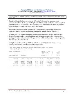
e categorical and continuous variables Thus handout will explain the difference between the two With binary in dependent variables marginal effects measure discrete

Upload by marina-yarberry
Published on 2014-12-01

Presentation Embed Code

<iframe width="560" height="315" src="https://www.docslides.com/embed/19403" frameborder="0" allowfullscreen></iframe>

Download Presentation

Download Presentation The PPT/PDF document "Marginal Effects for Continuous Variable..." is the property of its rightful owner. Permission is granted to download and print the materials on this web site for personal, non-commercial use only, and to display it on your personal computer provided you do not modify the materials and that you retain all copyright notices contained in the materials. By downloading content from our website, you accept the terms of this agreement.