/
EPS Colloquium, Harvard Cambridge, MA EPS Colloquium, Harvard Cambridge, MA

EPS Colloquium, Harvard Cambridge, MA - PowerPoint Presentation

maxasp
maxasp . @maxasp
Follow
344 views
Uploaded On 2020-07-03

EPS Colloquium, Harvard Cambridge, MA - PPT Presentation

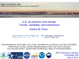
May 5 2014 83520601 Arlene M Fiore Acknowledgments Olivia Clifton Gus Correa Nora Mascioli Lee Murray Luke Valin CULDEO Harald Rieder U Graz Austria Elizabeth Barnes CSU ID: 794729

air climate regional change climate air change regional model ozone rcp8 ppb 2009 2006 usa 2013 surface cm3 gfdl

Share:

Link:

Embed:

Download Presentation from below link

Download The PPT/PDF document "EPS Colloquium, Harvard Cambridge, MA" is the property of its rightful owner. Permission is granted to download and print the materials on this web site for personal, non-commercial use only, and to display it on your personal computer provided you do not modify the materials and that you retain all copyright notices contained in the materials. By downloading content from our website, you accept the terms of this agreement.


Presentation Transcript

Slide1

EPS Colloquium, Harvard

Cambridge, MA

May 5, 2014

83520601

Arlene

M.

Fiore

Acknowledgments: Olivia Clifton,

Gus Correa, Nora

Mascioli

, Lee Murray, Luke

Valin

(CU/LDEO),

Harald

Rieder

(U Graz, Austria),

Elizabeth Barnes (CSU), Alex Turner (Harvard)Larry Horowitz (GFDL), Vaishali Naik (UCAR/GFDL), Meiyun Lin (Princeton/GFDL)

U.S. air pollution and climate: Trends, variability, and interactions

Haze over Boston, MA

http

://

www.airnow.gov

/

index.cfm?action

=particle_health.page1#3

Slide2

Ozone and Particulate Matter (PM)

are the top two U.S. air pollutants

Millions of people living in counties with air quality concentrations above the level of the U.S. National Ambient Air Quality StandardsOne or more NAAQS

Ozone (8-hour)

PM2.5 (annual/24-hr)

PM

10 (24-hr)

SO

2 (1-hr)

PM10

(24hr)

Lead (3-month)

NO

2 (annual/1-hr)

CO (8-hr)

0 20 40 60 80 100 120 140 160

2012

142.2133.228.216.1

15.1

8.1

EPA, 2014: http

://

www.epa.gov

/

airtrends

/

aqtrends.html#comparison

Slide3

IPCC

AR5 WG1 SPM

(2013)

A

ir pollutants and their precursors contribute to

climate forcing from preindustrial to present

Regulated in U.S.

a

s precursors

to ground-level O

3

A

nthropogenic

greenhouse gases methane + tropospheric ozone together contribute

~1/2 (abundance) to 2/3 (emissions) of

CO

2 radiative forcing (Lifetimes must also be considered: CO2

dominates long-term)

Net cooling from aerosols opposes

GHG warming

Warming

 Cooling

Slide4

Ground-level O

3 is photochemically

produced from regional sources (natural + anthrop.) that build on background levelsO3

+

CH

4

CO

NMVOC

NO

x

Fuel local-to-regional ozone

pollution episodes

Raise background ozone levels

Slide5

Exceeds

s

tandard

(24% of sites)

The U.S. ozone smog problem is spatially widespread

http://

www.epa.gov

/

airtrends

/2011/index.html

4

th

highest

maximum daily 8-hr average (MDA8) O3 in 2010

High-O3

events typically

occur in-- densely populated areas (sources)-- summer

(favorable meteorology)FUTURE? Lower threshold (60-70 ppb

[Federal Register, 2010]) would greatly expand non

-attainment regions

Estimated benefits from a ~1 ppb decrease in surface O

3

:

~ $1.4 billion (agriculture, forestry, non-mortality health) within U.S.

[

West and Fiore, 2005

]

~ 500-1000 avoided annual premature mortalities within N. America

[

Anenberg

et al., 2009]

Slide6

Trends in summer daytime (11am-4pm)

average ozone at rural U.S. monitoring sites (CASTNet): 1990 to 2010

Cooper et al., JGR, 2012Success in decreasing highest levels, but baseline rising (W. USA)Decreases in EUS attributed in observations and models to

NO

x emission controls in late 1990s, early 2000s [e.g., Frost et al., 2006

; Hudman et al., 2007

; van der

A. et al., 2008; Stavrakou

et al., 2008; Bloomer et al., 2009, 2010; Fang et al., 2010]

significant

n

ot significant

95%

5%

p

pb yr

-1

Slide7

The “tightening vise”

of ozone management

Ozone concentration

Historical

Future

(alternate view)

Hemispheric

background

Regional

Local

Standard

Future

Keating, T. J., J. J. West, and A. Farrell (2004) Prospects for international management of intercontinental air pollutant transport, in A. Stohl, Ed.,

Intercontinental Transport of Air Pollution

, Springer, p. 295-320.

 Future may require concerted efforts to lower background

Slide8

I

mplies that changes

in climate will influence air quality

Observations at U.S. EPA

CASTNet

site Penn State, PA 41N, 78W, 378m

July mean MDA8 O

3

(ppb)

Surface temperature

and

O3

are correlated on daily to inter-annual time scales in polluted regions

[e.g., Bloomer et al., 2009; Camalier et al., 2007; Cardelino and Chameides, 1990; Clark and Karl, 1982; Korsog and Wolff, 1991]

10am-5pm avg

pollutant sources

Degree of mixing

1. Meteorology (e.g., air stagnation)

What drives the observed O

3

-Temperature correlation?

T

NO

x

T-sensitive

NO

x

reservoir

NMVOCs

Deposition

2. Feedbacks (

Emis

,

C

hem

,

Dep

)

Slide9

Models estimate a ‘climate

change penalty’ (+2 to 8 ppb) on surface O3 over

U.S. but often disagree in sign regionally

Uncertain regional climate responses (and feedbacks) to global warming

M

odel estimates typically based on a few years of present and future (often 2050s) meteorology from 1 realization of 1 GCM

Modeled changes in summer mean of daily max 8-hour O

3 (ppb; future – present)

NE MW WC GC SE

Weaver et al., BAMS, 2009

ppbv

Wu et al.,

JGR

, 2008:

“Climate Penalty”

Slide10

‘First-look’ future projections with current chemistry-climate models for N. Amer. Surface O3 (emissions + climate change)

V.

Naik

, adapted

from

Fiore

et al.,

2012;

Kirtman

et al., 2013 (IPCC WG1

Ch

11)

RCP8.5

RCP6.0

RCP4.5

RCP2.6

D

ecadal time slice simulations(2-12 models)

A major advance to have coupled atmospheric chemistry in climate models

Trends mainly reflect ozone precursor emission pathways

A

nnual, continental-scale means reveal little about drivers of regional change

Multi-

model

Mean

Range across

ACCMIP CCMs

Multi-model Mean

Range across

CMIP5 CCMs

North America

Annual mean spatially averaged (land only) O

3

in surface air

T

ransient

simulations

(4 models

)

Slide11

How and why might extremes change?

Mean

shiftsVariabilityincreasesSymmetrychanges

Figure SPM.3, IPCC SREX 2012

http://ipcc-wg2.gov/SREX/

How do different

processes influence the overall distribution?

Meteorology (e.g., stagnation vs. ventilation)

 Shift in mean?

 Change in symmetry?

Changing global emissions (baseline)

Changing regional emissions (episodes)

Feedbacks (

Emis

,

C

hem

, Dep)

Does climate forcing from air pollutants influence regional climate extremes?

Aerosols vs. greenhouse gases

How do changes in the balance of these processes alter the seasonal cycle?

NE US: regional photochemistry (summer)

vs. transported background

Slide12

Approach: Targeted sensitivity simulations in a chemistry-climate model to examine chemistry-climate interactions

Tool: GFDL CM3 chemistry-climate model

~2°x2° horizontal resn.; 48

vertical levels

Over 6000 years of climate simulations that include chemistry (air quality) Options for nudging to re-analysis + global high-res ~50km

2

[Lin et al., 2012ab; 2014

]

Donner et al., J. Climate, 2011;

Golaz

et al., J. Climate,

2011;

John et al., ACP, 2012Turner et al., ACP, 2012Levy et al., JGR, 2013 Naik

et al., JGR, 2013 Barnes & Fiore, GRL, 2013

O

3

+

CH

4

CO

NMVOC

NO

x

Emission

(CH

4

abundance) pathways prescribed

Biogenic emissions held

constant

Lightning

NO

x

source tied to model meteorology

O

3

, (aerosols, etc.), affect simulated climate

Slide13

Approach: Historical + Future global change scenarios & targeted sensitivity simulations in GFDL CM3 CCM

Scenarios developed by CMIP5 [Taylor et al., BAMS, 2012]

in support of IPCC AR5 [e.g., Cubasch et al., 2013; Ch 1 WG 1 IPCC (see Box 1.1)]Preindustrial control (perpetual 1860 conditions >800 years)

(2) Historical (1860-2005) [

Lamarque et al., 2010] All forcings (5 ensemble members)

Greenhouse gas only (3)Aerosol only (3)

(3) Future (2006-2100): Representative Concentration Pathways

(+ perturbations)

 evaluate with observations

RCP8.5 (3)

RCP4.5 (3)

Percentage change: 2005 to 2100

Global

CO2

GlobalCH

4

GlobalNOx

NE USANOx CMIP5/AR5 [van Vuuren, 2011; Lamarque et al., 2011; Meinshausen et al., 2011] Isolate role of warming climate

 Quantify role of rising CH4 (vs. RCP8.5)

RCP8.5_WMGG (3)RCP4.5_WMGG (3)

RCP8.5_2005CH4

Slide14

In polluted (high-NOx

) regions, surface O3

typically peaks during summer(monthly averages at 3 NE USA measurement sites) Feb Apr Jun Aug Oct Dec

Monthly 1991-1996 averages across 3 NE USA sites

Clean Air Status and Trends Network (CASTNET)

Regionally

Representative sites

[

Reidmiller

et al., ACP, 2009

]

O. Clifton

Slide15

Shifting surface ozone seasonal cycle evident in observations over NE USA

Feb Apr Jun Aug Oct Dec

Monthly averages across 3 NE USA sites Clean Air Status and Trends Network (CASTNET)

Regionally

Representative sites

[

Reidmiller

et al., ACP, 2009

]

O. Clifton

Summer ozone decreases; shift towards broad spring-summer maximum

following EUS

NO

x

controls (“

NO

x SIP Call”)

1991-19962004-2009

Slide16

Structure of observed changes in monthly mean ozone captured by GFDL CM3 CCM (despite mean state bias)

Feb Apr Jun Aug Oct Dec

Monthly averages across 3 NE USA sites

Regionally

Representative sites

[

Reidmiller

et al., ACP, 2009

]

O. Clifton et al., submitted

OBS (

CASTNet

)CM3 (Model)

1991-1996

2004-2009

CM3 NE US shows summer O

3

decrease, small winter increase from ~25%

decrease in

NO

x

emissions

(

applied year-round)

[see also EPA, 2014;

Parrish

et al., GRL,

2013 find shifts at remote sites]

Slide17

Reversal of surface O3 seasonal cycle occurs in model under scenarios with dramatic regional NOx reductions

2005 to 2100 % change

CH

4

Global NO

x

NE USA

NOx

NE USA evolves from “polluted” to “background” over the 21

st

C

Reversal occurs after 2020s (not shown)

Clifton et al., submitted

2006-2015

2006-2015

2091-2100

2091-2100

RCP4.5

RCP8.5

Feb Apr Jun Aug Oct Dec

?

Decreasing

NO

x

emissions

lower summer O

3

3 ensemble

members for each scenario

Slide18

Doubling of global CH4 abundance (RCP8.5) raises NE USA surface ozone in model; largest impact during winter

Feb Apr Jun Aug Oct Dec

Doubling of methane increases surface O3

background by 6-11 ppb

2006-2015

2006-2015

2091-2100

2091-2100

RCP8.5_2005CH4

RCP8.5

Clifton et al., submitted

Slide19

“Climate penalty” on monthly mean NE USA surface O3 as simulated with the GFDL CM3 model

Feb Apr Jun Aug Oct Dec

JJA NE USA Temp (sfc) +2.5ºC

Feb Apr Jun Aug Oct Dec

2006-2015

2006-2015

2091-2100

2091-2100

RCP8.5_WMGG

RCP4.5_WMGG

JJA NE USA Temp (

sfc

) +

5

.5ºC

“Penalty” limited to

increases during warmest months

Extends

into May and September in high warming

scenario

Fully offset by regional precursor emission reductions under RCPs

Clifton et al., submitted

Slide20

How and why might air pollution extremes change?

Mean

shifts

Variability

increases

Symmetrychanges

Figure SPM.3, IPCC SREX 2012

http://ipcc-wg2.gov/SREX/

How do different

processes influence the overall distribution?

Meteorology (e.g., stagnation vs. ventilation)

 Shift in mean?

 Change in symmetry?

Changing global emissions (baseline)

Changing regional emissions (episodes)

Feedbacks (

Emis

,

C

hem, Dep)

Does climate forcing from air pollutants influence regional climate extremes?

Aerosols vs. greenhouse gases

How do changes in the balance of these processes alter the seasonal cycle?

NE US: regional photochemistry (summer)

vs. transported background

[

not today]

Slide21

Under RCPs, NE USA high-O3 summertime events decrease; beware ‘penalty’ from rising methane (via background O3

)

2006-2015

2016-2025

2026-2035

2036-2045

2046-2055

2056-2065

2066-2075

2076-20852086-2095

RCP4.5:Moderate

warming

Time

RCP8.5:

Extreme

warming

Time

RCP8.5

RCP4.5

2005 to 2100 % change

CH

4

Global

NO

x

NE USA

NO

x

Rising CH

4

in

RCP8.5

partially offsets O

3

decreases otherwise attained with regional

NO

x

controls (

RCP4.5

)

H.

Rieder

June-July-August GFDL CM3 MDA8 O

3

(ppb)

Slide22

GFDL CM3 generally captures NE US JJA surface O

3 decrease following NOx emission controls (-25% early 1990s to mid-2000s)

Rieder et al., in prepImplies bias correction based on present-day observations can be applied to scenarios with NOx changes (RCPs for 21

st

C) Focus on upper half of distribution

Observed(CASTNet

)

GFDL CM3 Model

JJA MDA8 O3

(ppb)

Relative Frequency

Slide23

Characterizing observed ‘extreme’ ozone pollution events

JJA MDA8 O

3

1987-2009 at

CASTNet Penn State site

Gaussian (ppb)

Observed MDA8 O3 (ppb)

Observed MDA8 O3 (ppb)

Generalized Pareto Distribution Model (ppb)

EVT Approach:

(Peak-over-threshold)for MDA8 O3

>75 ppb

Gaussian:

Poor fitfor extremes

1988-

1998

1999-2009

Rieder et al., ERL 2013 Extreme Value Theory (EVT) methods describe the high tail of the observed ozone distribution (not true for Gaussian)

Slide24

EVT methods enable derivation of probabilistic “return levels” for JJA MDA8 O

3

within a given “return period”CASTNet site: Penn State, PA

Rieder

et al., ERL 2013

1988-

1998

1999-2009

Sharp decline in return levels

from 1988-1998 to 1999-2009; longer return periods for a given event

(attributed to

NO

x emission controls)Consistent with prior work [

e.g., Frost et al., 2006; Bloomer et al., 2009, 2010]

New approach to translates air pollution changes into probabilistic language

Apply methods to 23 EUS

CASTNet sites to derive1-year return levels Decreased by 2-16 ppb

 Remain above 75 ppb

Slide25

Large NOx reductions offset climate penalty on O3

extremes1-year Return Levels in CM3 chemistry-climate model (corrected)

Summer (JJA) MDA8 Surface O3

ppb

2046-2055

RCP4.5_WMGG:

Pollutant emissions held constant (2005) +

c

limate warming

2091-2100

RCP4.5:

Large

NO

x

decreases +

climate warming

All at or below 60 ppbNearly all at or below 70 ppbRieder

et al., in prep We find a simple relationship between

NOx reductions

and 1-year return levels

Slide26

A mechanism underlying ‘climate penalty’: Frequency

of NE US summer storms decreases as the planet warms…

RCP4.5RCP8.5 (1 ens. member)

Turner et al., ACP, 2013

Region for counting storms

Region for counting O

3

events

Number of storms per summer in the GFDL CM3 model,

as determined from applying

the MCMS storm tracker [

Bauer et al., 2013] to 6-hourly sea level pressure fields

(follows approach of Leibensperger

et al., 2008)(3 ens. members)

Trends are significant relative to variability in preindustrial control simulation

Slide27

…but the storm count – O3 event relationship is weaker than derived from observations

Detrended O

3

pollution daysDetrended

Number of mid-latitude cyclones

Observed relationship

[Leibensperger et al, ACP, 2008]

Slope = -4.2 O

3 events/storm

1980-2006:

NCEP/NCAR Reanalysis 1 & AQS ozone

Simulated relationship (GFDL CM3)

[Turner et al., ACP, 2013]

Model problem (bias/process representation)?

Change in drivers (under warming climate)?Decadal variability in strength of relationship?

RCP4.5_WMGG 2006-2100 Can we find a simpler diagnostic of large-scale circulation changes?

Slope = -2.9 O3

events/storm

Slide28

Peak latitude of summertime surface O

3 variability over Eastern N. America

follows the jet (500 hPa) as climate warmsBarnes & Fiore, GRL, 2013

Each point = 10 year mean (over ensemble members)

RCP4.5_WMGG

 Decadal variabilityRelevance to shorter periods?

Differences in model jet position lead to inter-model differences in AQ response?

O

3

-Temperature relationship (not shown)

a

lso aligns with jet latitude

 Historically observed relationships may not hold if large-scale circulation shifts

Latitude of max std. dev. of JJA MDA8 O3 (deg N)

RCP8.5: most warming,

Largest jet shift

RCP8.5

jet: 2086-2095

jet: 2006-2015

c

hange in O

3

std. dev. (ppb)

Slide29

How and why might air pollution extremes change?

Mean

shifts

Variability

increases

Symmetrychanges

Figure SPM.3, IPCC SREX 2012

http://ipcc-wg2.gov/SREX/

How do different

processes influence the overall distribution?

Meteorology (e.g., stagnation vs. ventilation)

 Shift in mean?

 Change in symmetry?

Changing global emissions (baseline)

Changing regional emissions (episodes)

Feedbacks (

Emis

,

C

hem, Dep)

Does climate forcing from air pollutants influence regional climate extremes?

Aerosols vs. greenhouse gases

How do changes in the balance of these processes alter the seasonal cycle?

NE US: regional photochemistry (summer)

vs. transported background

[

not today]

Slide30

Offsetting impacts on extreme temperature events from greenhouse gases vs. aerosol over historical period

N. Mascioli

-4.0 -2.0 0.0 2.0 4.0

Change in Hottest Days (°C)

Greenhouse Gas Only

Aerosol Only

Consistent (?) patterns (spatial correlation r = 0.56 )

Pollutants

 regional weather events

 extreme pollution?

Single forcing historical simulations in GFDL CM3 (all other forcings held at 1860 conditions)

(1976-2005) – (1860-1889)

(annual maximum daily temperature [

e.g., Sillman et al., 2013ab])

X = outside range of variability (95%) of differences between 30-year intervals in

preind. control simulation

Slide31

Increase in hottest days projected throughout 21st Century under extreme warming scenario

N. Mascioli

 Amplified warming during extreme events from aerosol removal?

Preferred response patterns?

-4.0 -2.0 0.0 2.0 4.0

Change in Hottest Days (°C)

-8.0 -4.0 0.0 4.0

8

.0

Change in Hottest Days (°C)

(annual maximum daily temperature [

e.g.,

Sillman

et al., 2013ab])

GFDL CM3 1 ensemble member, RCP8.5 scenario: aerosols decline, GHGs rise

mid-21stC: (2035-2065) – (2006-2036)

late-21stC: (2070-2100) – (2006-2036)

X = outside range of variability (95%) of differences between 30-year intervals in preind. control simulation

Slide32

Atmospheric Chemistry Group at LDEO/CU

On the roof of our building following mid-Dec snowfall(missing from photo: undergraduate researcher Jean Guo)

Harald Nora

Gus

Arlene

Luke

Olivia

Lee

Slide33

U.S. air pollution and climate: Trends

, variability, and interactions

Relevant to model differences in O3 response to climate? [Weaver et al., 2009; Jacob & Winner, 2009; Fiore

et al., 2012

]

Zonal O

3 variability aligns with the 500

hPa jet over NE NA (JJA)

Decadal jet shifts can influence O3

:T [Barnes & Fiore, 2013

]

NO

x

reductions reverse the O3 seasonal cycle over NE USA

Will NE US evolve to ‘background’ air quality over the 21st

C?

Detecting chemistry-climate interactions

Will (global) aerosol removal amplify response of U.S. climate extremes to rising GHGs?New approach to characterize pollution events [Rieder et al., 2013

]

Double ‘penalty’ on

NE US O

3

from

climate change + rising

CH

4

?

RCP4.5

Time

RCP8.5

Rising CH

4

+ decreasing

NO

x

shift balance of regionally produced vs. transported O

3

Time

Translation to probabilistic language,”1-year event”, useful for decadal planning?