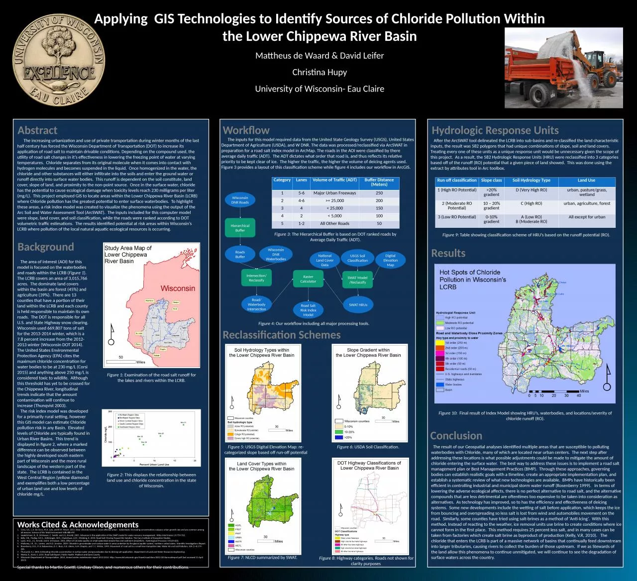
Abstract Applying GIS Technologies to Identify Sources of Chloride Pollution Within the - PowerPoint Presentation

1. AbstractApplying GIS Technologies to Identify Sources of Chloride Pollution Within the Lower Chippewa River BasinMattheus de Waard & David LeiferChristina HupyUniversity of Wisconsin- Eau Claire The increasing urbanization and use of private transportation during winter months of the last half century has forced the Wisconsin Department of Transportation (DOT) to increase its application of road salt to maintain drivable conditions. Depending on the compound used, the utility of road salt changes in it’s effectiveness in lowering the freezing point of water at varying temperatures. Chloride separates from its original molecule when it comes into contact with hydrogen molecules and becomes suspended in the liquid. Once homogenized in the water, the chloride and other substances will either infiltrate into the soils and enter the ground water or runoff directly into surface water bodies. This runoff is dependent on the soil constitute, land cover, slope of land, and proximity to the non-point source. Once in the surface water, chloride has the potential to cause ecological damage when toxicity levels reach 230 milligrams per liter (mg/L). This project employed GIS to locate areas within the Lower Chippewa River Basin (LCRB) where Chloride pollution has the greatest potential to enter surface waterbodies. To highlight these areas, a risk index model was created to visualize the phenomena using the output of the Arc Soil and Water Assessment Tool (ArcSWAT). The inputs included for this computer model were slope, land cover, and soil classification, while the roads were ranked according to DOT volumetric traffic estimations. The results identified potential at risk areas within Wisconsin’s LCRB where pollution of the local natural aquatic ecological resources is occurring.Workflow The inputs for this model required data from the United State Geology Survey (USGS), United States Department of Agriculture (USDA), and W DNR. The data was processed/reclassified via ArcSWAT in preparation for a road salt index model in ArcMap. The roads in the AOI were classified by there average daily traffic (ADT). The ADT dictates what order that road is, and thus reflects its relative priority to be kept clear of ice. The higher the traffic, the higher the volume of deicing agents used. Figure 3 provides a layout of this classification scheme while figure 4 includes our workflow in ArcGIS. The area of interest (AOI) for this model is focused on the waterbodies and roads within the LCRB (Figure 1). The LCRB covers an area of 3,015,766 acres. The dominate land covers within the basin are forest (45%) and agriculture (39%). There are 13 counties that have a portion of their land within the LCRB and each county is held responsible to maintain its own roads. The DOT is responsible for all U.S. and State Highway snow clearing. Wisconsin used 669,807 tons of salt for the 2013-2014 winter, which is a 7.8 percent increase from the 2012-2013 winter (Wisconsin DOT 2014). The United States Environmental Protection Agency (EPA) cites the maximum chloride concentration for water bodies to be at 230 mg/L (Corsi 2015) and anything above 250 mg/L is considered toxic to wildlife. Although this threshold has yet to be crossed for the Chippewa River, longitudinal trends indicate that the amount contamination will continue to increase (Thunqvist 2003). The risk index model was developed for a primarily rural setting, however this GIS model can estimate Chloride pollution risk in any Basin. Elevated levels of Chloride are typically found in Urban River Basins. This trend is displayed in figure 2, where a marked difference can be observed between the highly developed south eastern part of Wisconsin and the more rural landscape of the western part of the state. The LCRB is contained in the West Central Region (yellow diamond) and exemplifies both a low percentage of urban land use and low levels of chloride mg/L.Figure 1: Examination of the road salt runoff for the lakes and rivers within the LCRB.BackgroundCorsi, S.R., L.A. De Cicco, M.A. Lutz, and R.M. Hirsch. 2015. River chloride trends in snow-affected urban watersheds: increasing concentrations outpace urban growth rate and are common among all seasons. Science of the Total Environment 508:488-497.Jayakrishnan, R., R. Srinivasan, C. Santhi, and J.G. Arnold. 2005. Advances in the application of the SWAT model for water resource management. Wiley InterScience 19:759-763.Kelly, V.R., Findlay, S.E.G., Schlesinger, W.H., Chatrchyan, A.M., Menking, K. 2010. Road Salt: Moving Toward the Solution. The Cary Institute of Ecosystem Studies.Luzio, M.D., J.G. Arnold, and R. Srinivasan. 2005. Effect of GIS data quality on small watershed stream flow and sediment simulations. Hydrological Processes 19:629-650. Mullaney, J.R., D.L. Lorenz, and A.D. Arnston. 2009. Chloride in groundwater and surface water in areas underlain by the glacial aquifer system, northern united states. Scientific Investigations Report.Rosenberry, D.O., P. A. Bukaveckas, D. C. Buso, G.E. Likens, A.M. Shapiro, and T. C. Winter, 1999, Movement of road salt to a small New Hampshire lake. Water Air and Soil Pollution, 109 (1-4):179-206.Thunqvist, E.J. 2003. Estimating chloride concentration in surface water and groundwater due to deicing salt application. Department of Land and Water Resources Engineering. Wenta, R., Kirsti, S. 2014, Road Salt Report. Public Health: Madison and Dane County.Wisconsin Department of Transportation. 2014. Annual winter maintenance report 2013-2014. http://www.dot.wisconsin.gov/travel/road/docs/2013-2014annualreport.pdf (last accessed 21 April 2015).Special thanks to Martin Goettl, Lindsay Olson, and numerous others for their contributions.National Land Cover DataUSGS Soil ClassificationDigital Elevation MapSWAT Model /ReclassifyRoad/ Waterbody IntersectionSWAT HRUsRaster CalculatorRoad Salt Risk Index ModelWisconsin DNR RoadsHierarchical BufferRoads BufferWisconsin DNR WaterbodiesIntersection/ReclassifyFigure 2: This displays the relationship between land use and chloride concentration in the state of Wisconsin.Figure 5: USGS Digital Elevation Map: re-categorized slope based off run-off potentialFigure 6: USDA Soil Classification.Figure 7: NLCD summarized by SWAT.Figure 8: Highway categories. Roads not shown for clarity purposes Conclusion The result of our Geospatial analyses identified multiple areas that are susceptible to polluting waterbodies with Chloride, many of which are located near urban centers. The next step after addressing these locations is what possible adjustments could be made to mitigate the amount of chloride entering the surface water. The best way to address these issues is to implement a road salt management plan or Best Management Practices (BMP). Through these approaches, governing bodies can establish realistic goals with a timeline, create an appropriate implementation plan, and establish a systematic review of what new technologies are available. BMPs have historically been efficient in controlling industrial and municipal storm water runoff (Rosenberry 1999). In terms of lowering the adverse ecological affects, there is no perfect alternative to road salt, and the alternative compounds that are less detrimental are oftentimes too expensive to be taken into consideration as alternatives. As technology has improved, so to has the efficiency and effectiveness of deicing systems. Some new developments include the wetting of salt before application, which keeps the ice from bouncing and overspreading so less salt is lost from wind and automobiles movement on the road. Similarly, some counties have tried using salt-brines as a method of ‘Anti-Icing’. With this method, Instead of reacting to the weather, ice removal units use brine to create conditions where ice cannot form in the first place. This method requires 25 percent less salt, and in many cases can be taken from factories which create salt brine as byproduct of production (Kelly, V.R, 2010). The chloride that enters the LCRB is part of a massive network of basins that continually feed downstream into larger tributaries, causing rivers to collect the burden of those upstream. If we as Stewards of the land allow this phenomena to continue unmitigated, we will continue to see the degradation of surface waters across the country.CategoryLanesVolume of Traffic (ADT)Buffer Distance (Meters)15-6Major Urban Freeways25024-6>= 25,00020034< 25,00015042< 5,00010051-2All Other Roads50Figure 3: The Hierarchical Buffer is based on DOT ranked roads by Average Daily Traffic (ADT).Reclassification SchemesHydrologic Response Units After the ArcSWAT tool delineated the LCRB into sub-basins and re-classified the land characteristic inputs, the result was 582 polygons that had unique combinations of slope, soil and land covers. Treating every one of these units as a unique response unit would be unnecessary given the scope of this project. As a result, the 582 Hydrologic Response Units (HRU) were reclassified into 3 categories based off of the runoff (RO) potential that a given piece of land showed. This was done using the extract by attributes tool in Arc toolbox.Run off classificationSlope classSoil Hydrology TypeLand Use 1 (High RO Potential)>20% gradientD (Very High RO)urban, pasture/grass, wetland2 (Moderate RO Potential)10 – 20% gradientC (High RO)urban, agriculture, forest3 (Low RO Potential)0-10%gradientA (Low RO)B (Moderate RO)All except for urbanFigure 9: Table showing classification scheme of HRU’s based on the runoff potential (RO).Figure 10: Final result of Index Model showing HRU’s, waterbodies, and locations/severity of chloride runoff (RO).Figure 4: Our workflow including all major processing tools.Works Cited & Acknowledgements Results