/
Scaling Relationships in Biology Scaling Relationships in Biology

Scaling Relationships in Biology - PowerPoint Presentation

melody
melody . @melody
Follow
65 views
Uploaded On 2023-09-25

Scaling Relationships in Biology - PPT Presentation

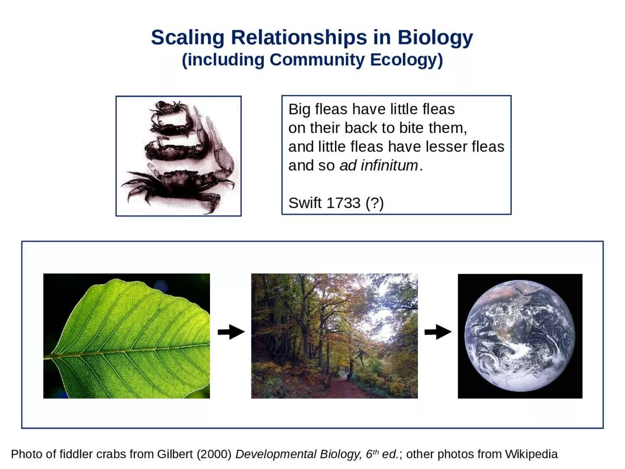
including Community Ecology Big fleas have little fleas on their back to bite them and little fleas have lesser fleas and so ad infinitum Swift 1733 Photo of fiddler crabs from Gilbert 2000 ID: 1021365

relationships scaling area amp scaling relationships amp area community function log10 surface size density volume relationship length areay scales

Share:

Link:

Embed:

Download Presentation from below link

Download Presentation The PPT/PDF document "Scaling Relationships in Biology" is the property of its rightful owner. Permission is granted to download and print the materials on this web site for personal, non-commercial use only, and to display it on your personal computer provided you do not modify the materials and that you retain all copyright notices contained in the materials. By downloading content from our website, you accept the terms of this agreement.


Presentation Transcript

1. Scaling Relationships in Biology(including Community Ecology)Big fleas have little fleason their back to bite them, and little fleas have lesser fleasand so ad infinitum.Swift 1733 (?)Photo of fiddler crabs from Gilbert (2000) Developmental Biology, 6th ed.; other photos from Wikipedia

2. Scaling RelationshipsStatistic from West et al. (1997); Fig. from Bonner (1988)Organisms range over 21 orders of magnitude in body size!

3. Scaling RelationshipsFigure from Levin (1992)Biologically relevant processes operate over an enormousrange of spatial & temporal scales

4. Scaling RelationshipsPhotos from WikipediaProcesses are naturally linked across scales, so how can we extrapolatefrom one scale to another (e.g., leaf  forest  globe)?What are the mechanistic links among patterns and processes across scales?For example… gas exchange through individual stomata & global warming represent phenomena that occur at vastly different scales of space & time

5. Scaling RelationshipsA good starting point is to identify scaling relationshipsScaling often assesses how attributes changewith changes in a fundamental dimension (e.g., length, mass, time)The attributes of the organism, community or ecosystem are generally the dependent variables (Y), whereas the fundamental dimensionis the independent variable (X)

6. Scaling RelationshipsMany scaling relationships can be expressed as power laws:Y = c XsX is the independent variable – measured in units of a fundamental dimension; c is a constant of proportionality;and s is the exponent (or “power” of the function)The relationship is a straight line on a log-log plot:Log10(Y) = Log10(c) + s  Log10(X)…and by rearranging, this is the form of the familiar equation for a straight line:y = mx + b

7. Scaling RelationshipsArea = Length2Area  Length2Volume = Length3Volume  Length3Surface area = 6 * Length2Surface area  Length2Consider the scaling of squares & cubes as functions of the length of a side (the fundamental dimension)

8. AreaY = X2(accelerating function)LengthScaling Relationships

9. AreaY = X2(accelerating function)LengthScaling Relationships

10. AreaY = X2(accelerating function)LengthScaling Relationships

11. Etc…Log10(Area)AreaY = X2(accelerating function)Y = 2XLengthLog10(Length)Scaling Relationships

12. LengthLog10(Length)Log10(Surface Area)Surface areaEtc…Y = 2X + 0.778Y = 6 * X2(accelerating function)Scaling Relationships

13. Log10(Volume)VolumeEtc…Y = X3(accelerating function)Y = 3XLengthLog10(Length)Scaling Relationships

14. Scaling RelationshipsSurface area = 4  r2Surface area  r2Volume = 4/3  r3Volume  r3Consider the ways in which surface area & volumeof a sphere scale with its radius

15. Scaling RelationshipsSurface-to-volume ratio: Surface area  r2  Surface area1/2  r Volume  r3  Volume1/3  rSurface area1/2  Volume1/3  Surface area  Volume2/3

16. Etc…Log10(Volume)Log10(Surface area)VolumeSurface areaY=4.83 * X0.667(decelerating function)Volume increases proportionately faster than surface areaY=0.667 * X + 0.68Slope = 1Scaling Relationships

17. Etc…VolumeSurface areaY=4.83 * X0.667(decelerating function)This simple fact has myriad important implications for biology(e.g., Bergmann’s “rule”?)Log10(Volume)Log10(Surface area)Y=0.667 * X + 0.68Slope = 1Scaling Relationships

18. Etc…VolumeSurface areaY=4.83 * X0.667(decelerating function)For example, endoparasite S should increase more rapidly than ectoparasite S as host body size increasesLog10(Volume)Log10(Surface area)Y=0.667 * X + 0.68Slope = 1Scaling Relationships

19. Etc…Y = 3 * X-1RadiusSurface area / VolumeAs you could infer from the earlier figures, the surface area to volume ratio changes with the radius of the sphereScaling Relationships

20. Etc…Log10(Surface area / Volume)Y = 3 * X-1RadiusSurface area / VolumeLog10(Radius)Y= -1 * X + 0.48…and the rate of change of the ratio is constant in log-log plotting spaceScaling Relationships

21. Scaling RelationshipsAllometry – Coined by Julian Huxley (1932) for the study of size& its relationship to characteristics within individuals(due to ontogenetic changes) & among organisms(due to size-related differences in shape, metabolism, etc.)For example, size is related allometrically to basal metabolic rate in birds & mammals:B  M3/4The red line’s slope = 1

22. Scaling Relationships in Community EcologyFigure from West et al. (1997)Metabolic Ecology TheoryGeoff West, James Brown & Brian Enquist proposed that many allometric relationships in biology are governed by the physical properties of branching distribution networks (e.g., blood vessels, xylem & phloem)

23. Scaling RelationshipsAllometric relationship: Height vs. diameter in treesThe critical buckling height for cylinders is:Hcritical = k * (E/)1/3 * D2/3GiantsequoiaDouglasfirPonderosapineTherefore, if trees maintain “elastic similarity”:H  D2/3See Greenhill (1881); Figure from McMahon (1975)

24. Scaling RelationshipsAllometric relationship: Height vs. diameter in treesIf trees maintain “elastic similarity”:H  D2/3Dataset for U.S. record trees.Both lines have slopes = 2/3;the broken line is 1/4 the magnitude of the complete lineTrees avoid buckling under their own weight, with a 4x safety factorSee Greenhill (1881); Figure from McMahon (1975)

25. Scaling Relationships in Community EcologySpecies-area relationshipsThe Arrhenius equation describes apower-law scaling relationship:S = cAzlog (S) = log (c) + z * log (A)Figure from Rosenzweig (1995)

26. Scaling Relationships in Community Ecologya. Insular races of mammals compared to their nearest mainland relatives; the scaling relationship suggests an “optimum size of 100 g” Figure from Brown’s Macroecology (1995)Mainland vs. islandsize relationships (Foster’s “rule”)

27. Scaling Relationships in Community Ecologya. Insular races of mammals compared to their nearest mainland relatives; the scaling relationship suggests an “optimum size of 100 g” b. The largest (solid circles) & smallest (open circles) mammals of a landmass as a function of area; as area – and thus the number of species – decreases, the sizes of the mammals converge on 100 gFigure from Brown’s Macroecology (1995)Mainland vs. islandsize relationships (Foster’s “rule”)

28. Scaling Relationships in Community EcologySize vs. density in plant communitiesThe relationship between size & number for plants grown in monoculture gave rise to the empirical “self-thinning rule”, i.e., the mean size of individuals in the stand is proportional to their density raised to the -3/2 power Self-thinning rule:m = k N -3/2Plantago asiaticaFigure from Yoda et al. (1963)

29. Scaling Relationships in Community Ecology Density-1  Mass2/3 Mass  Density-3/2The similarity to geometric constraints suggested this possibility:Size vs. density in plant communitiesSelf-thinning rule:m = k N -3/2Plantago asiatica Area  Volume2/3 Area  Density-1 Volume  MassFigure from Yoda et al. (1963)

30. Scaling Relationships in Community EcologySize vs. density in plant communitiesEnquist & colleagues have challenged the traditional -3/2 thinning rule by re-examining size-density relationships & by providing a new, mechanistic way to approach the problem Enquist et al.’s prediction:m = k N -4/3Figure from Enquist et al. (1998)

31. Scaling Relationships in Community EcologySize vs. density in plant communitiesEnquist & Niklas (2001) suggested Metabolic Ecology Theory as the explanation for the apparent consistency of size-density relationships across forestsTheir predictiontranslates into:N = k DBH -2Figure from Enquist & Niklas (2001)

32. 110100100011010010001000010000001000000Diameter (mm)N / km2Empirical curves do not exactly match predictions (slope = -2; shaded region) from Metabolic Ecology Theory (Enquist & Niklas 2001 )Scaling Relationships in Community EcologyFigure redrawn from Muller-Landau, Condit, Harms et al. (2006) Ecology Letters

33. Scaling Relationships in Community EcologySpecies-genus & species-family ratiosEnquist et al. (2001) suggested three hypotheses for the relationship between species richness and number of higher taxa within a local communityc. Communities could be scattered within the shaded region below the constraint line, such that the variance in abundance of higher taxa increases with S; higher taxa abundance would be effectively unpredictable from Sa. A positive relationship with a shallow slope; as species are added they come from an increasingly limited subset of higher taxa b. A slope of unity represents the upper constraint boundary; addition of new species occurs only upon addition of higher taxaFigure from Enquist et al. (2002)

34. Scaling Relationships in Community EcologyFigure from Enquist et al. (2002)Species-genus & species-family ratiosEnquist et al. (2001) found surprising similarity among tropical forests worldwide

35. Scaling Relationships – FractalsFigure from West et al. (1997)Fractal models describe the geometry of a wide variety of natural objectsE.g., the branching distribution networks of organisms…Within an object, as a fundamental dimension changes, fractal properties of the object obey scaling (power function) relationships

36. If you are curious, visit: http://www.arcytech.org/java/fractals/sierpinski.shtmlThe Sierpinski TriangleScaling Relationships – FractalsFractal objects may also exhibit the property of self similarity(self-similar objects maintain characteristic properties over all scales)

37. Scaling Relationships – Fractals“In the natural world, there is no guarantee that… elegant self-similar properties will apply” Sugihara & May (1990)Even so, fractal properties (and self-similarity over finite scales) appear throughout the natural world:Barnsley’s fractal fern

38. Scaling Relationships – Fractals“In the natural world, there is no guarantee that… elegant self-similar properties will apply” Sugihara & May (1990)Even so, fractal properties (and self-similarity over finite scales) appear throughout the natural world:Clematis fremontii –Fremont’s leather flower;endemic to KS, NE, MO(Original from Erickson 1945)Figure from Brown’s Macroecology (1995)

39. Scaling Relationships – FractalsIt has become customary to introduce fractals with reference to measuring the coast of Britain (e.g., Mandelbrot 1983) , a project that first suggested the intriguing fact that as the scale of the ruler decreases, the length of the coast increases:L = K δ1-D L = Total length δ = Length of the ruler D = Fractal dimensionSelf-similarity characterizes the object of interest if D is constant over all scales (δ), i.e., if the power term of the function is constantFigure from Sugihara & May (1990)

40. Scaling Relationships – FractalsThe fractal dimension (D) can be thought of as the “crookedness,” “tortuosity” or “complexity” of the object:(d)D = 1D = 1.26D = 1.5D = 2Figure from Sugihara & May (1990)

41. Scaling Relationships – FractalsIn practice there are many ways to estimate D, and to use D in community ecology (see Sugihara & May 1990).Morse et al. (1985) used the boundary-grid method to show that the areas of leaf surfaces in nature display fractal properties, and that D changes with δD ≈ 1.5 for the boundaries of vegetation surfacesMorse et al. (1985) show that this means that for an order of magnitude decrease in body length, there is 3.16 more area to occupy!Figure from Morse et al. (1985, Nature)

42. Morse et al. (1985), used their analysis to suggest an explanation for the observation that as the body sizes of arthropods increase, their numbers (densities) decrease more rapidly than expected if available area remained constantScaling Relationships – FractalsFigure from Morse et al. (1985, Nature)