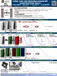
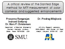
PPT-A critical review of the Slanted Edge method for MTF measurement of color cameras and PowerPoint Presentation

Prasanna Rangarajan Indranil Sinharoy Dr Marc P Christensen Dr Predrag Milojkovic Department of Electrical Engineering Southern Methodist University Dallas

Upload by min-jolicoeur
Published on 2018-11-09

Presentation Embed Code

<iframe width="560" height="315" src="https://www.docslides.com/embed/723928" frameborder="0" allowfullscreen></iframe>

Download Presentation

Download Presentation The PPT/PDF document "A critical review of the Slanted Edge me..." is the property of its rightful owner. Permission is granted to download and print the materials on this web site for personal, non-commercial use only, and to display it on your personal computer provided you do not modify the materials and that you retain all copyright notices contained in the materials. By downloading content from our website, you accept the terms of this agreement.