Summary Statistics Notation n X th Measures of Central Location Mean xxx N xxx In practice - PDF document

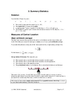
��(c) 2006; 2016B. Gerstmansumstats.docxPage of 3: Summary StatisticsNotationConsider these 10 ages (in years)The symbol )290(101x The distinction between the sample mean (denoted ) and population mean (denoted µ) is critical to your future understanding of statistical inferenc . ixnx1 ��(c) 2006; 2016B. Gerstmansumstats.docxPage of Reporting the mean: The mean should be roundedto three (or at most four) significant digits before reportingin order to avoid an appearance of pseudoprecision. In addition, units of measure should be included when reporting the mean.For example, the mean of our data is yearsMedian The median was covered in the previous chapter. Briefly, this is the value with a depthof in the ordered arrayWhen is odds, this will fall on a value in the dataset. When is even, this will fall between two values. Here are the sizes of 5 benign tumors (cubic centimeters): The median has a depth of (5 + 1) / 2 = 3 and a value oe median isslightly moreresistant to outliers. This means it resists the pull of outliers and is more apt to stay put. For instance, if the biggest value in the above set had been mistakenly entered 120 instead of 12, the mean would shift from 8.4 to 30 but the median would stay put at The mode is the most frequently occurring value in a data set. The mode is unreliable iall but very large data sets. ��(c) 2006; 2016B. Gerstmansumstats.docxPage of Comparison of the Mean, Median, and ModeThe mean, median, and mode are equivalent when the distribution is unimodal and symmetrical. However, with asymmetry, the median is approximately onethird the distance between the mean and mode:The mean, median, and mode offer different advantages and disadvantages. The mean offers the advantages of familiarity and efficiency. It also has advantages when making inferences about a population mean. On the downside, the mean is markedly influenced by extreme skewness and outliers. Under circumstances of extreme skewness, the median is a more “stable.” An often cited example of this advantage come when considering the salary of employees, where the salary of highly paid executives skews the average income toward a misleadingly high value. Another example is the average price of homes, in which case high priced homes skew the data in a positive direction. In such circumstances, the median is less likely to be misinterpreted, and is therefore the preferred measure of central location.You can judge the asymmetry of a distribution by comparing its mean and median. When the mean is greater than the median, the distribution has a positive skew. When the mean is about equal to the median, the distribution is symmetrical. When the mean is less than the median, the distribution has a negative skew:mean� median positive skewmean median symmetrymean median negative skewIn general, the mean is preferred when data are symmetrical and do not have outliers. In other instances, the median may be the preferred measure of central location. ��(c) 2006; 2016B. Gerstmansumstats.docxPage of Measures of SpreadRangeSimply noting the minimum and maximum values can be useful when describing the spread of distribution. However, calculating the sample range (maximum minimum) is not an acceptablemeasure of spreadbecause t will consistently underestimate he population rangepoint summariesand quartilesThe point summary consists ofQ0 ≡ Quartile 0(the minimumQ1 ≡ Quartile 1(bigger than 25% of the data points)Q2 ≡ Quartile 2 (the median)Q3 ≡ Quartile 3 (bigger than 75% of the data points)Q4 ≡ Quartile 4(the maximumThe median is called 2 because it is equal to or greater than quarters of the data points. The minimum is Q0 because it is greater than or equal to zeroquarters of the data points. You get it.When the data set is large (>=100), it is easy to find Q1 and Q3. With small data sets, the exact location of quartiles must be interpolatedThe two most common methods of interpolation for this purpose are weighted averages and Tukey’s hinges.To find Tukey’s hingesPut the data in rank order ocate the median of the data set. Divide the data set into two groups: a low group and a high group. When is odd, the median should be placed in both groups. Find the ‘median’of the low group. This is Q1.Find the ‘median’ of the high group. This is Q3.xample #1. Consider thisordered array = 10) The low group has a ‘median’ of 21. This is Q1. The high group has a ‘median’ of This is Q3.he fivepoint summary 27.5, 42, 52xample #2. Consider this new ordered array Recall thatyou must include the median in both the low group and high groupfor Tukey’s hingesherefore the low group consists of {1.47, 2.06, 2.36, 3.43}. The medianof this low group (Q1) is the average of 2.06 and 2.36, or 2.21.The medianof the high group (Q3) is 3.76. The five point summary is 1.47, 2.21, 3.43, 3.76, 3.95 ��(c) 2006; 2016B. Gerstmansumstats.docxPage of Interquartile range (IQR)An measure of spreadesp.for asymmetrical datais the interquartile range (IQR):IQR = Q3 − Q1The IQR for Example #1 (prior page) = 42 21 = 21. or Example #2 (prior page), IQR= 3.76 2.21 = 1.55. Our IQRs are also called hingespreadsecause they quantify the spread from the lower hingeto the upper hingeandwhiskers plotsoxplots)Tukeyot consistsof a box showing Q1, Q2, and Qwhiskersand, occasionallytside valuesAfter determining the 5 point summary and IQR for a dataset, then alculate(but do not draw) fencesas followsFenceLower= Q1 − (1.5)(IQR)FenceUpper= Q3 + (1.5)(IQR)Note that the fences ar1.5 hingespreads above below the hingesDo not plot these fences.Any value that is above the upper fence is an upper outside value. Any values below the lower fence is a lower outside value. Plot these points, if any, on the graph. The largest value still inside the upper fence is the upper inside value. The smallest value still inside the lower fence is the lower inside value. Drawn whiskersfrom the upper hinge to the upper inside valueand from the bottom hinge to the lower inside value. Boxplot example #1. The 5 - point summary ( determine on prior page ) is ( 5, 21, 27.5, 42, 52) . The box extends from 21 to 42 and has a line in its midst to identify the median at 27.5.he = 21 (1.5)(21) = and = 42 + (1.5)(21) = 73.5. No values in the data set are bove or elow refore, there are outside values. The upper inside value is 52 and the lower inside is the 5. Whiskers are drawn from the hinges to the inside values.The boxplot isshown on the next page. ��(c) 2006; 2016B. Gerstmansumstats.docxPage of Interpretation of boxplots.Think shape, location and spread. Shape easist to onsiderin terms of symmetry and potential outiers. Is the median about halfway between the hinges? Is the box bout halfway between the whiskers? Outside values are potential outliers. The cenral location be summarized by the median and box, which is the middle 50% of valuesSpread quantified in terms of the hingespreadand whiskerspreadThe boxplot for example is fairly symmetrical and has no outside valueshe a medianthat is a little less than 30 and a hingespread is from 21 to 42.New exampleHere’s a new set of values The five - point summary is ( 3, 22, 25.5, 29, 51 ). IQR = 29 ㈲  㴀′㤠⬀ ⠀ㄮ㔩⠀㜀⤀‽″㤮㔮⁆㴀′㈠(1.5)(7) = 11.5.There is one value above the upper fence (51). There is one value below the lower fence (3). The largest value still inside the upper fences (upper inside value) is 31. The smallest value still inside the lower fence (lower inside value) is 21 ��(c) 2006; 2016B. Gerstmansumstats.docxPage of Standard Deviation and VarianceBoth thestandard deviation and variance are based ondeviation), defined asquare each deviation in the dataset and sum theto derive the sum of squares ( 2)(xxSSi The sample variance is the meansum of squares: SSns112 Note: The denominator in this formula is by− 1, not This is necessary to derive an unbiased estimate of the population variance. The number − 1 is called the degree of freedomThe sample standard deviationis simply the square root of the variance: 2ss Illustrative example. Recall the10 ages21, 42, 5, 11, 30, 50, 28, 27, 24, The sample mean x is 29.0(page 1). The variance is calculated i Values ( x i ) D eviations ( d i ) Sqyared d 2 1 21 21 – 29 = – 8 – 8 2 = 64 2 42 42 – 29 = 13 13 2 = 169 3 5 5 – 29 = – 24 – 24 2 = 576 4 11 11 – 29 = – 18 −18 㴀″㈀㐀 ㈹ 㴀‱ ㈹ 㴀′㄀ 㴀‴㐀㄀ ㈹‽  ㈹‽  ㈹‽  㴠㈀㔀 ㈹ 㴀′㌀ 㴀‵㈀㤀 匀甀浳 卵洀昀⁓焀甀愀爀攀猀  2134 The sample variance is 1111.237110213412nSSs years[Note the squared units.]The standard deviation 398.151111.2372ss = 15.4 years.Report the standard deviation in conjunction with the mean, round accordingly, and include units of measure. “The mean age of the participants was 29.0 years with a standard deviationof 15.4 years. Calculating a few variance and standard dev iations by hand is instructive. However, most of the time we calculate the standard deviation with a computer or calculator o not need to calculate variances and standard deviations by hand unless t he instructions specifically request a step - by - step cal culation.