PDF-University of Salford: Clinical Gait Analysis 3.1

Author : mitsue-stanley | Published Date : 2016-08-21

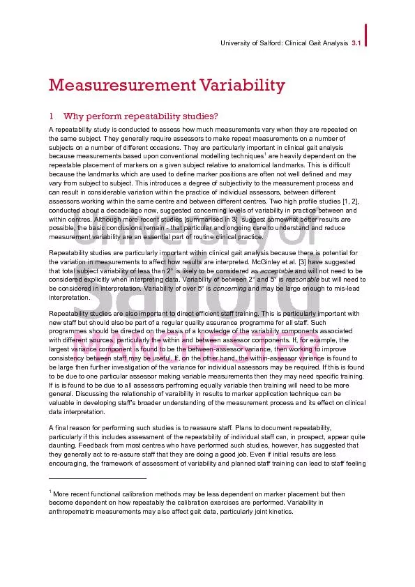
Measuresurement Variability Why perform repeatability studies A repeatability study is conducted to assess how much measurements vary when they are repeated on the

Presentation Embed Code

<iframe width="560" height="315" src="https://www.docslides.com/embed/453085" frameborder="0" allowfullscreen></iframe>

Download Presentation

Download Presentation The PPT/PDF document "University of Salford: Clinical Gait Ana..." is the property of its rightful owner. Permission is granted to download and print the materials on this website for personal, non-commercial use only, and to display it on your personal computer provided you do not modify the materials and that you retain all copyright notices contained in the materials. By downloading content from our website, you accept the terms of this agreement.

University of Salford: Clinical Gait Analysis 3.1: Transcript

Download Document

Here is the link to download the presentation.
"University of Salford: Clinical Gait Analysis 3.1"The content belongs to its owner. You may download and print it for personal use, without modification, and keep all copyright notices. By downloading, you agree to these terms.