Dr Ron Lembke Operations Management How much do we have Design capacity max output designed for Everything goes right enough support staff Effective Capacity Routine maintenance Affected by resources allocated ID: 181352
Download Presentation The PPT/PDF document "5. Capacity and Waiting" is the property of its rightful owner. Permission is granted to download and print the materials on this web site for personal, non-commercial use only, and to display it on your personal computer provided you do not modify the materials and that you retain all copyright notices contained in the materials. By downloading content from our website, you accept the terms of this agreement.
Slide1
5. Capacity and Waiting
Dr. Ron Lembke
Operations ManagementSlide2
How much do we have?
Design capacity: max output designed
for
Everything goes right, enough support staff
Effective Capacity
Routine maintenance
Affected by resources allocated
We
can only sustain so much effort.
Output
level process designed for
Lowest
cost per
unitSlide3
Loss of capacitySlide4
Utilization and Efficiency
Capacity
utilization =
actual output
design capacity
Efficiency = actual output
effective capacityEfficiency can be > 1.0 but not for long Slide5
Scenario 1
Design Capacity 140 tons
Effective Capacity 124 tons –
landing gear
could
fail in bad weather landing
With 120 ton loadUtilization: 120/140 = 0.857Efficiency: 120/124 = 0.968Slide6
Economies of Scale
Cost per unit cheaper, the more you make
Fixed costs spread over more unitsSlide7
Dis-economies of scale
Congestion, confusion, supervision
Running at 100 mph means more maintenance needed
Overtime, burnout, mistakesSlide8
Marginal Output of Time
Value of working
n
hrs is
Onda
As you work more hours, your productivity per hour goes down
Eventually, it goes negative.
Better to work b instead of e hrs
S.J. Chapman
,
1909, “Hours of
Labour
,” The Economic Journal 19(75) 353-373Slide9
Learning Curves
time/unit goes down
consistently
First 1 takes 15 min, 2
nd
takes 5, 3
rd
takes 3Down 10% (for example) as output doublesWe can use Logarithms to approximate thiscost per unit after 10,000 units?If you ever need this, email me, and we can talk as much as you
wantSlide10
Break-Even Points
FC = Fixed
Cost
VC
= variable cost per unit
Q
BE = Break-even quantityR = revenue per unit
FC+VC*Q
Volume, Q
R*Q
Break-Even
PointSlide11
Cost Volume Analysis
Solve for Break-Even Point
For profit of P,
Q
BE
= FC
R – VCFC = $50,000 VC=$2, R=$10QBE = 50,000 / (10-2) = 6,250 unitsSlide12
747-400 vs 777
Monthly Debt Operating $/ton mile
747 $1,367,000 $50,000 $1.45
777 $1,517,000 $50,000 $1.38
Break-even:
747 ($1,367,000+$50,000)/(2-1.45)=
2,576,364 ton/miles per month
777 ($1,517,000
+$50,000)/(2-1.38)= 2,527,419 ton/miles per monthSlide13
Capacity Tradeoffs
Can we make combinations in between?
150,000
Two-door cars
120,000
4-door
carsSlide14
Adjust for aircraft size
777
– 124 tons per flight
2,576,364/124 = 20,777 full miles/month
747
– 104 tons per flight
2,527,419/104 = 24,302 full miles/monthSlide15
# Flights / month
747:
20,777 miles/2,869
= 7.24 fully loaded flights
= 8 full flights
777:
24,302 miles/2,869
= 8.47 fully loaded flights= 9 full flightsSlide16
Time Horizons
Long-Range: over a year – acquiring, disposing of production resources
Intermediate Range: Monthly or quarterly plans, hiring, firing, layoffs
Short Range – less than a month, daily or weekly scheduling process, overtime, worker scheduling, etc.Slide17
Adding Capacity
Expensive to add capacity
A few large expansions are cheaper (per unit) than many small additions
Large expansions allow of “clean sheet of paper” thinking, re-design of processes
Carry unused overhead for a long time
May never be neededSlide18
Capacity Planning
How much capacity should we add?
Conservative Optimistic
Forecast possible demand scenarios (Chapter 11)
Determine capacity needed for likely levels
Determine “capacity cushion” desiredSlide19
Capacity Sources
In addition to expanding facilities:
Two or three shifts
Outsourcing non-core activities
Training or acquisition of faster equipmentSlide20
What Would Henry Say?
Ford introduced the $5 (per day) wage in 1914
He introduced the 40 hour work week
“so people would have more time to buy”
It also meant more output: 3*8 > 2*10
“Now we know from our experience in changing from six to five days and back again that we can get at least as great production in five days as we can in six, and we shall probably get a greater, for the pressure will bring better methods.
Crowther, World’s Work, 1926Slide21
Toyota Capacity
1997: Cars
and
vans?
That’s crazy talk
First time in North America
292,000 Camrys89,000 Siennas89,000 AvalonsSlide22
Decision Trees
Consider different possible decisions, and different possible outcomes
Compute expected profits of each decision
Choose decision with highest expected profits, work your way back up the tree.Slide23
Draw the decision treeSlide24
Everyone is Just Waiting
Everyone is just waitingSlide25
Retail Lines
Things you don’t need in easy reach
Candy
Seasonal, promotional items
People hate waiting in line, get bored easily, reach for magazine or book to look at while in
line
Deposit slips
Postal FormsSlide26
In-Line Entertainment
Set up the story
Get more buy-in to ride
Plus, keep from boredomSlide27
Disney FastPass
Wait without standing around
Come back to ride at assigned time
Only hold one pass at a time
Ride other rides
Buy souvenirs
Do more rides per daySlide28
Benefits of Interactivity
Slow me down before going again
Create buzz, harvest email addressesSlide29
False Hope
Dumbo
Peter PanSlide30
Queues
In England, they don’t ‘wait in line,’ they ‘wait on queue.’
So the study of lines is called queueing theory.Slide31
Cost-Effectiveness
How much money do we lose from people waiting in line for the copy machine?
Would that justify a new machine?
How much money do we lose from bailing out (balking)?Slide32
Service Differences
Arrival Rate very variable
Can’t store the products - yesterday’s flight?
Service times variable
Serve me “Right Now!”
Rates change quickly
Schedule capacity in 10 minute intervals, not months
How much capacity do we need?Slide33
We are the problem
Customers arrive randomly.
Time between arrivals is called the “interarrival time”
Interarrival times often have the “memoryless property”:
On average, interarrival time is 60 sec.
the last person came in 30 sec. ago, expected time until next person: 60 sec.
5 minutes since last person: still 60 sec.
Variability in flow means excess capacity is needed Slide34
Memoryless Property
Interarrival
time = time between arrivals
Memoryless
property means it doesn’t matter how long you’ve been waiting.
If average wait is 5 min, and you’ve been there 10 min, expected time until bus comes = 5 min
Exponential Distribution
Probability time is t = Slide35
Poisson Distribution
Assumes interarrival times are exponential
Tells the probability of a given number of arrivals during some time period T.Slide36
Simeon Denis Poisson
"Researches on the probability of criminal and civil verdicts" 1837
looked at the form of the binomial distribution when the number of trials was large.
He derived the cumulative Poisson distribution as the limiting case of the binomial when the chance of success tend to zero.
Slide37
Larger average, more normalSlide38
Queueing Theory Equations
Memoryless
Assumptions:
Exponential arrival rate =
= 10
Avg.
interarrival
time = 1/ = 1/10 hr or 60* 1/10 = 6 minExponential service rate = = 12Avg service time = 1/ = 1/12Utilization =
= /10/12 = 5/6 = 0.833Slide39
Avg. # of customes
L
q
=
avg
# in
queue = Ls
= avg # in system =Slide40
Probability of # in System
Probability of no customers in system
Probability of
n
customers in systemSlide41
Average Time
W
q
=
avg
time in the
queueWs = avg time in systemSlide42
Example
Customers arrive at your service desk at a rate of 20 per hour, you can help 35 per hr.
What % of the time are you busy?
How many people are in the
line,
on average?
How many people are
there in total, on avg?Slide43
Queueing Example
λ=20,
μ
=35 so
Utilization
ρ
=20/35 = 0.571
Lq = avg # in line =Ls
= avg # in system = Lq
+
/
= 0.762 + 0.571 = 1.332Slide44
How Long is the Wait?
Time waiting for service =
L
q
= 0.762, λ=20
Wq = 0.762 / 20 = 0.0381 hours Wq = 0.0381 * 60 = 2.29 minTotal time in system =
Wq = 0.0381 * 60 = 2.29 min μ=35, service time = 1/35 hrs = 1.714 min
W
s
= 2.29 + 1.71 = 4.0 min Slide45
What did we learn?
Memoryless
property means exponential distribution, Poisson arrivals
Results hold for simple systems: one line, one server
Average length of time in line, and system
Average number of people in line and in system
Probability of
n people in the system